A03-03 基础绘图系统

2017-05-27 19:16:25

作图流程

顺序

配置函数par: 指定版式和全局参数
底图函数: 初始化底图，将覆盖前一张底图
- plot, plot.new
- smoothScatter, barplot, boxplot, bxp, dotchart, hist, pie, stars
- pairs, spineplot, matplot, assocplot, coplot, cdplot, stripchart, sunflowerplot, mosaicplot, fourfoldplot, symbols
注释函数: 底图上覆盖其他元素
- 图: lines, abline, segments, points, pch, box, rect, curve, arrows, polygon, polypath, matlines, matpoints
- 文: title, legend, text, mtext
- 其他: axis, grid, rug

版面版式和全局配置

`par`

par()打印所有制图版式参数的当前取值
par("<参数>")打印某个特定参数的当前取值
par(<参数>=...)修改特定参数的取值

> par("mar")
[1] 5.1 4.1 4.1 2.1

> par(mar=c(5, 4, 4, 2))
> par("mar")
[1] 5 4 4 2

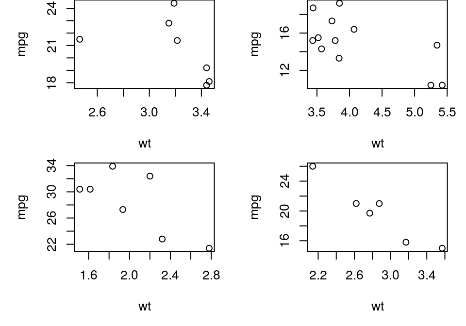
分面(facet)版式

外边距

mar: 向量c(下, 左, 上, 右)，单位是“行”
- 默认值: c(5, 4, 4, 2) + 0.1
mai: 向量c(下, 左, 上, 右)，单位是“英寸”
- 默认值: c(1.02, 0.82, 0.82, 0.42)

内边距

oma: 向量c(下, 左, 上, 右)，单位是“行”，默认值: c(0, 0, 0, 0)
omi: 向量c(下, 左, 上, 右)，单位是“英寸”，默认值: c(0, 0, 0, 0)
omd: c(x1, x2, y1, y2)，单位是相对于设备尺寸的"%"，默认值: c(0, 1, 0, 1)

美学参数

还有一些美学/视觉效果类参数。具体请查阅?par

bg: 背景色
cex: 注释图文的大小
family: 字体
fg: 前景色
font: 字体效果
lty: 线条的种类
lwd: 线宽
pch: 点的种类

基础底图

散点图 points

散点图: 两变量相关性。数据很多时，用smoothScatter

with(mtcars, plot(wt, mpg, type='p'))

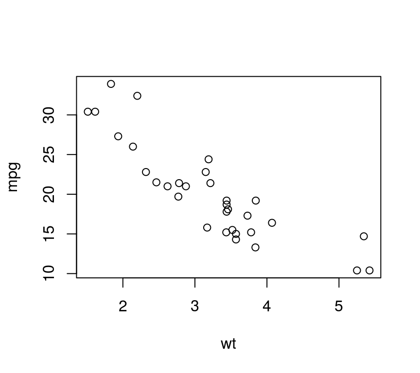
# 默认type='p'

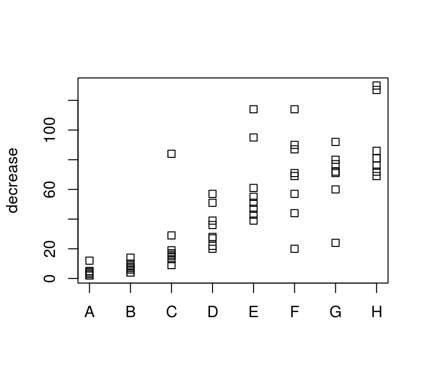
文本型变量作散点图

stripchart(decrease ~ treatment,
    vertical=TRUE, data=OrchardSprays)

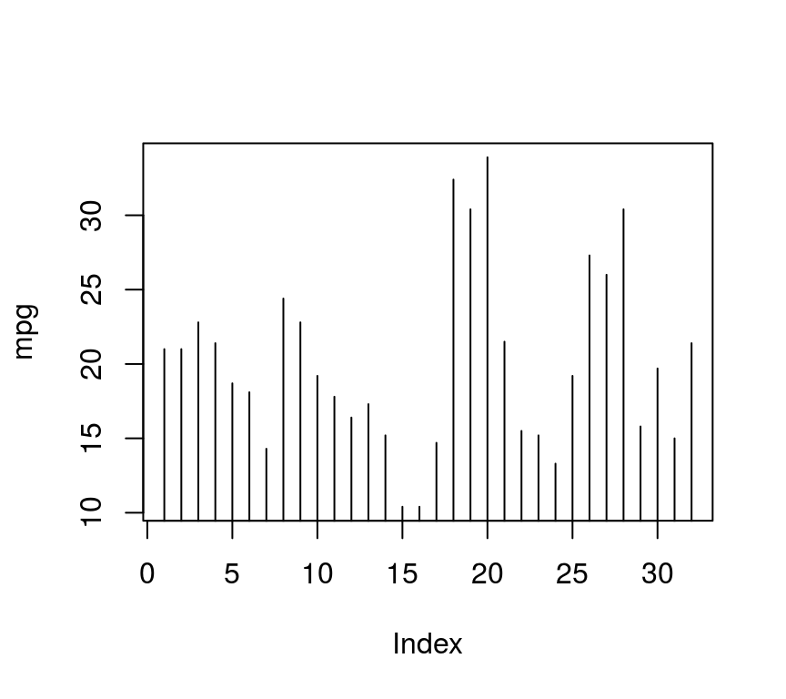
直方图 histogram

直方图: 单变量密度分布

with(mtcars, hist(mpg))

或用线段图

with(mtcars, plot(mpg, type='h'))

箱式图 boxplot

连续性变量的分布

boxplot(ToothGrowth$len)

多个箱式图

boxplot(len ~ dose, data = ToothGrowth)

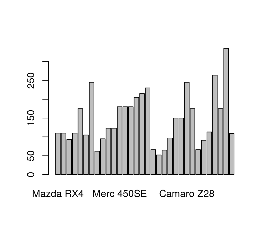
柱/条形图 barplot

分类变量的比较

hp <- mtcars$hp
names(hp) <- row.names(mtcars)
barplot(hp)

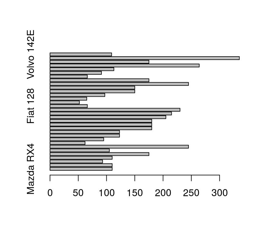
自变量较多时用横向条图

hp <- mtcars$hp
names(hp) <- row.names(mtcars)
barplot(hp, horiz=TRUE)

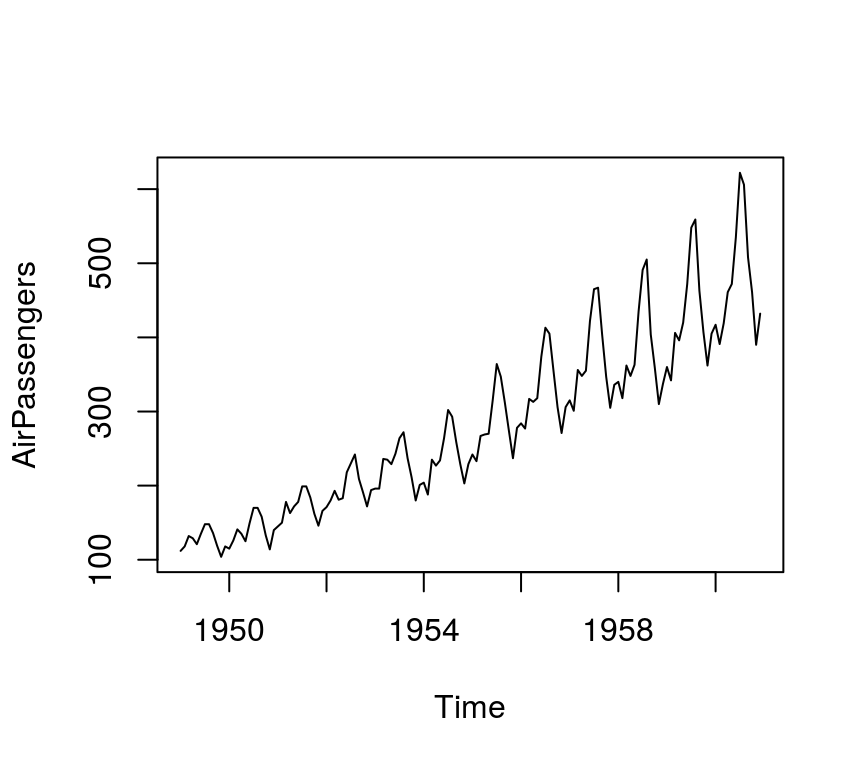
折线图 lines

表示趋势

plot(AirPassengers) # 时间序列数据默认type='l'

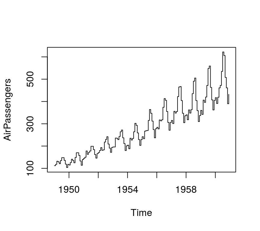
阶梯折线

plot(AirPassengers, type='s')  # 阶梯图

进阶底图

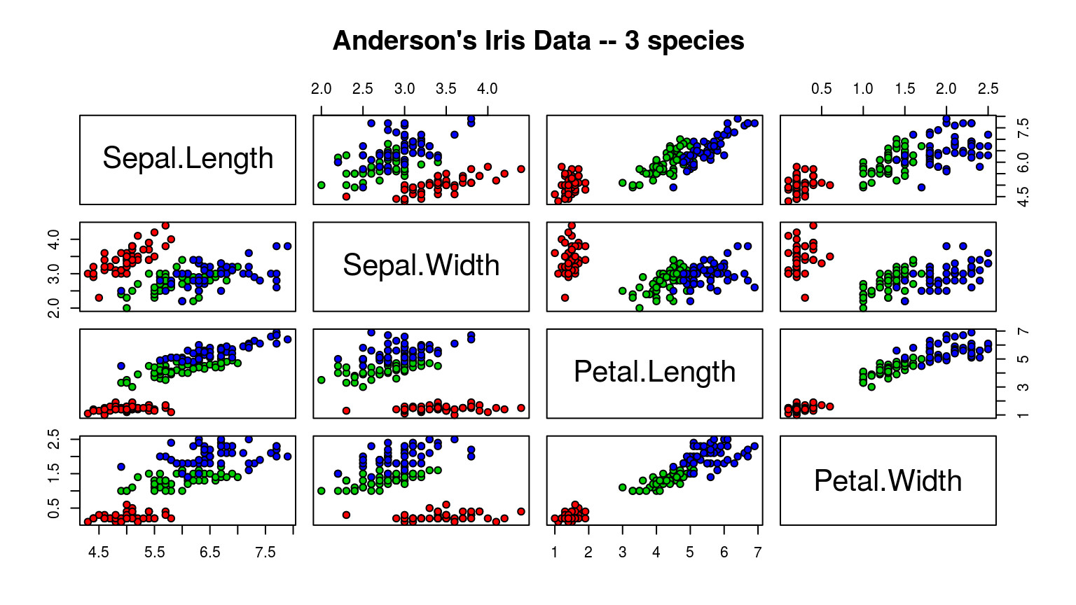
散点图矩阵 pairs

pairs(iris[1:4], main = "Anderson's Iris Data -- 3 species",
      pch = 21, bg = c("red", "green3", "blue")[unclass(iris$Species)])

跨矩阵的列比较图 matplot

iris.S=array(NA, dim=c(50, 4, 3),
             dimnames=list(NULL, colnames(iris)[-5], levels(iris$Species)))
for(i in 1:3) iris.S[,,i] <- data.matrix(iris[1:50+50*(i-1), -5])
matplot(iris.S[,"Petal.Length",], iris.S[,'Petal.Width',], pch="scv")

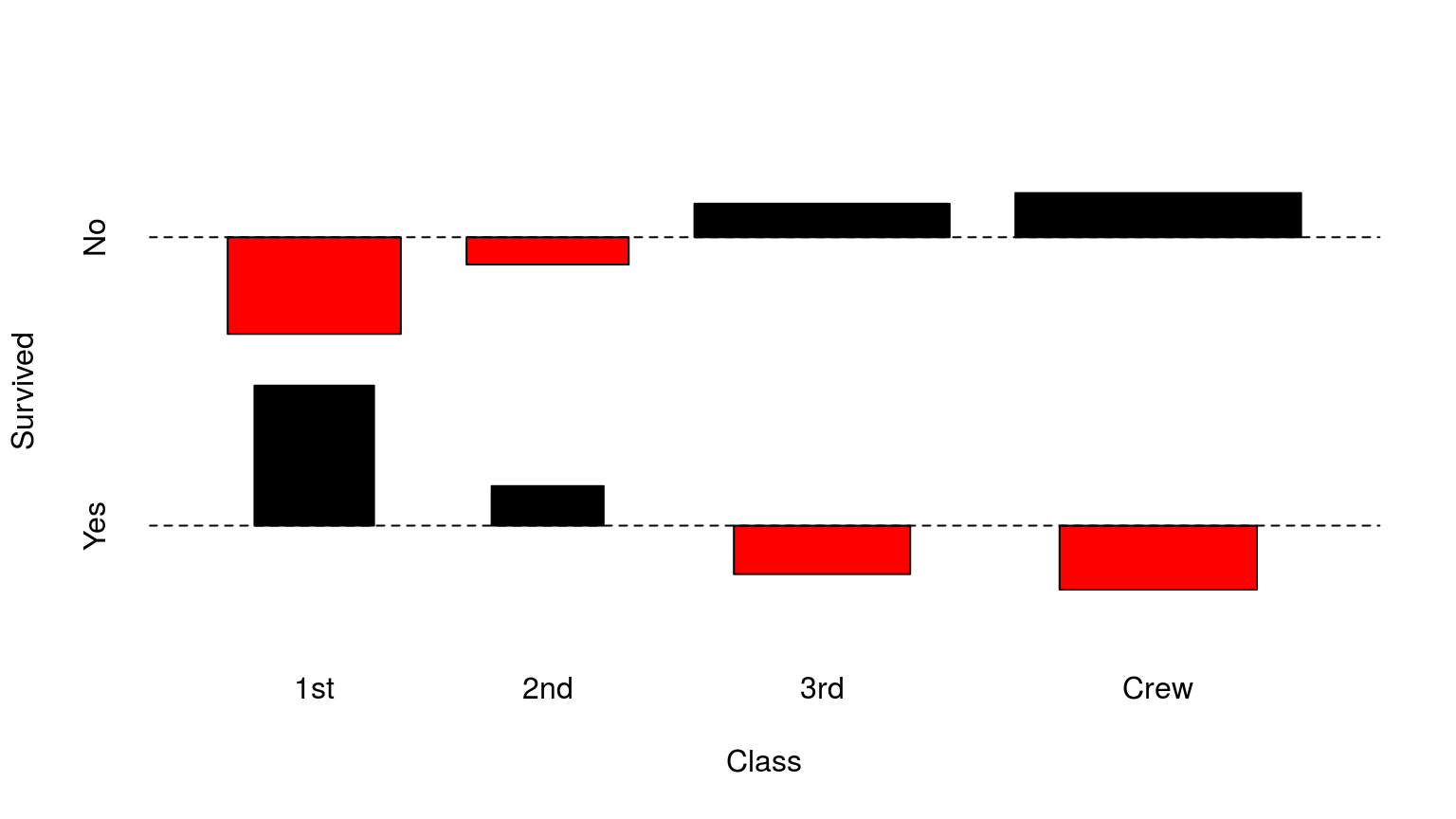
关联散点图 assocplot

x <- margin.table(Titanic, c(1,4))
assocplot(x)

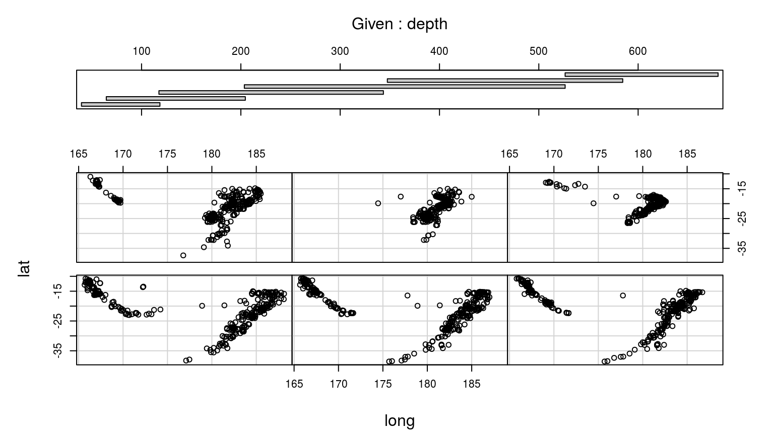
条件散点图 coplot

coplot(lat ~ long | depth, data = quakes)

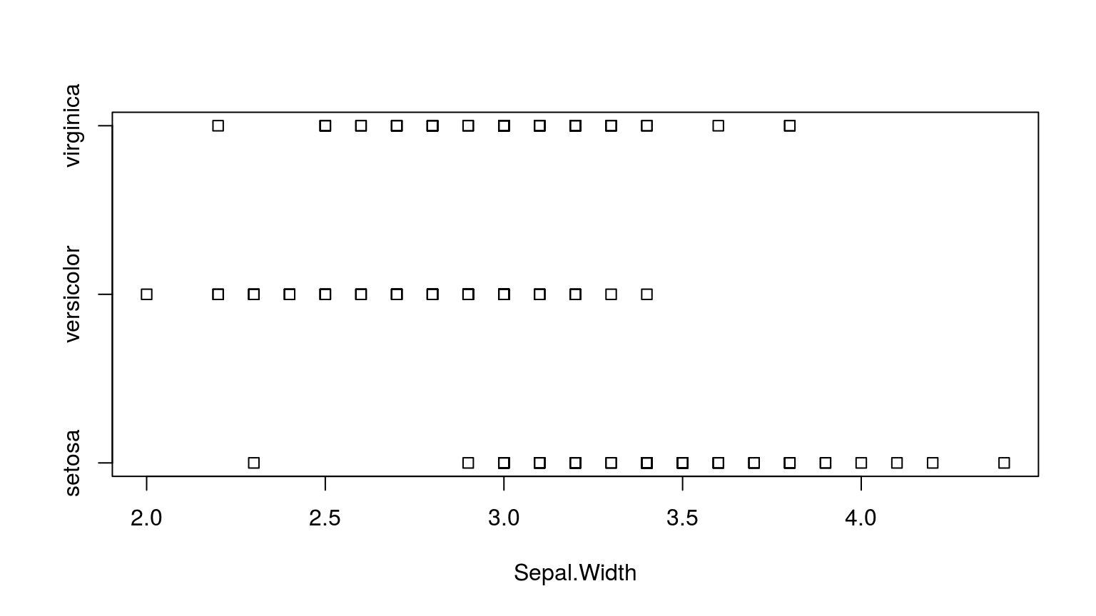
一维散点图 stripchart

with(iris, stripchart(Sepal.Width ~ Species))

向日葵图 sunflowerplot

sunflowerplot(iris[, 3:4])

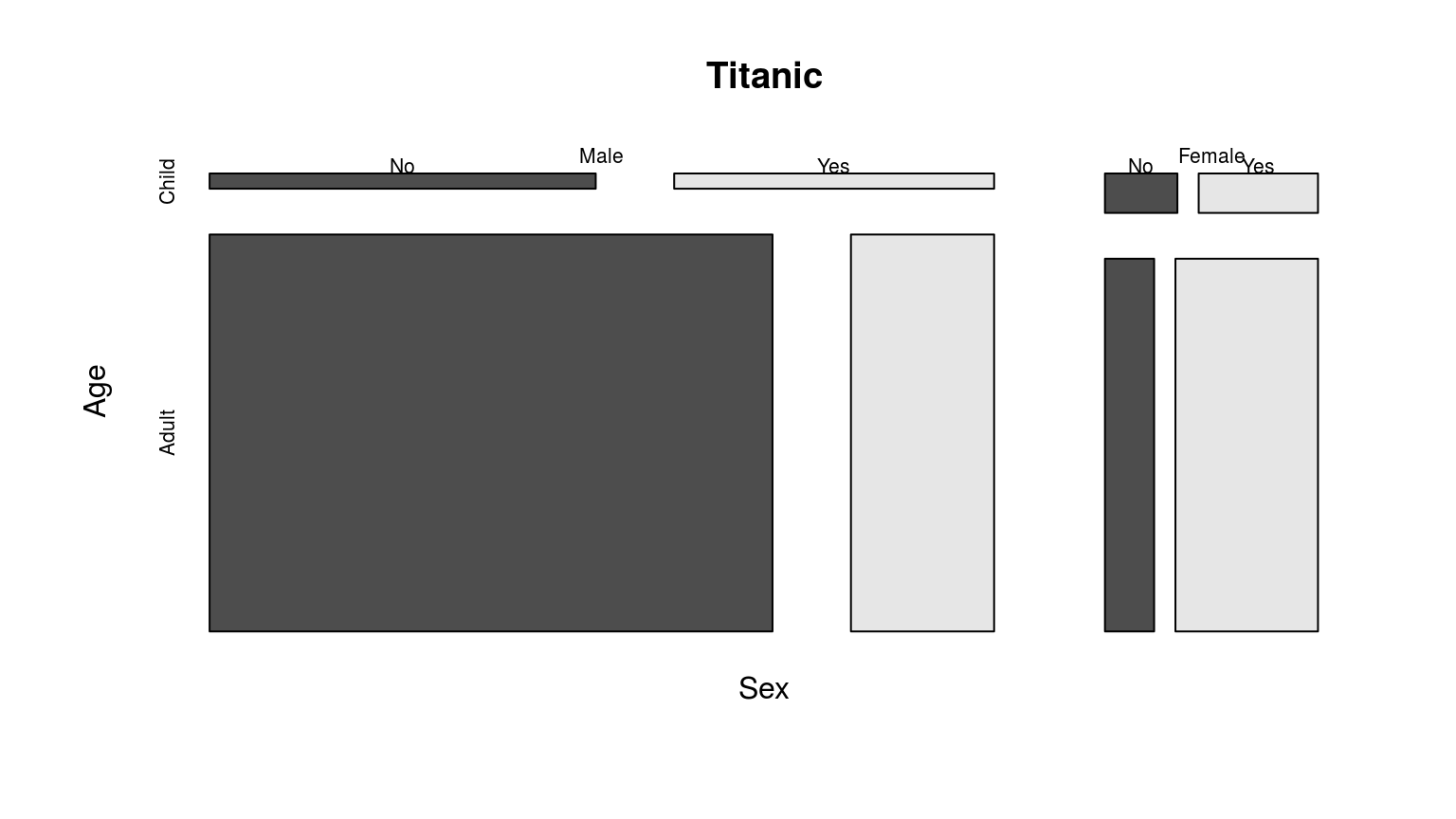
马赛克图 mosaicplot

mosaicplot(~ Sex + Age + Survived, data = Titanic, color = TRUE)

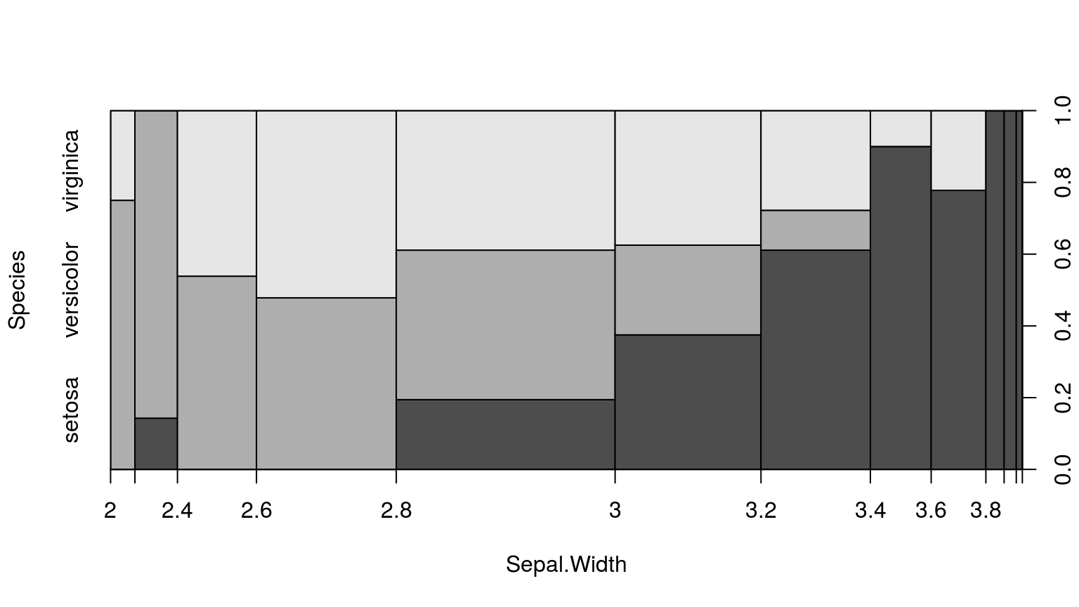
棘状图 spineplot

with(iris, spineplot(Species ~ Sepal.Width))

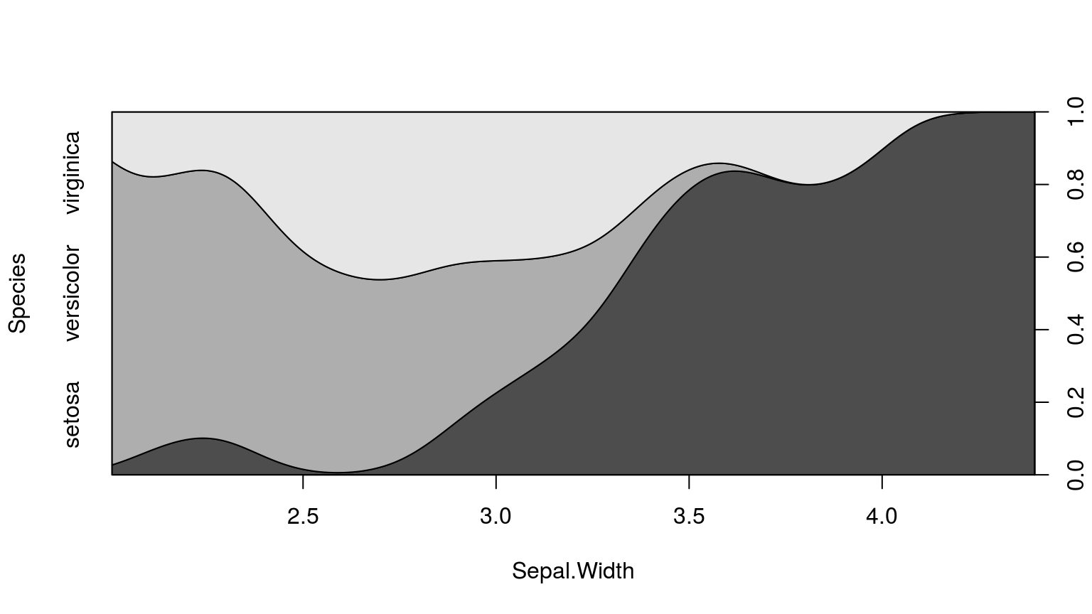
条件密度图 cdplot

with(iris, cdplot(Species ~ Sepal.Width))

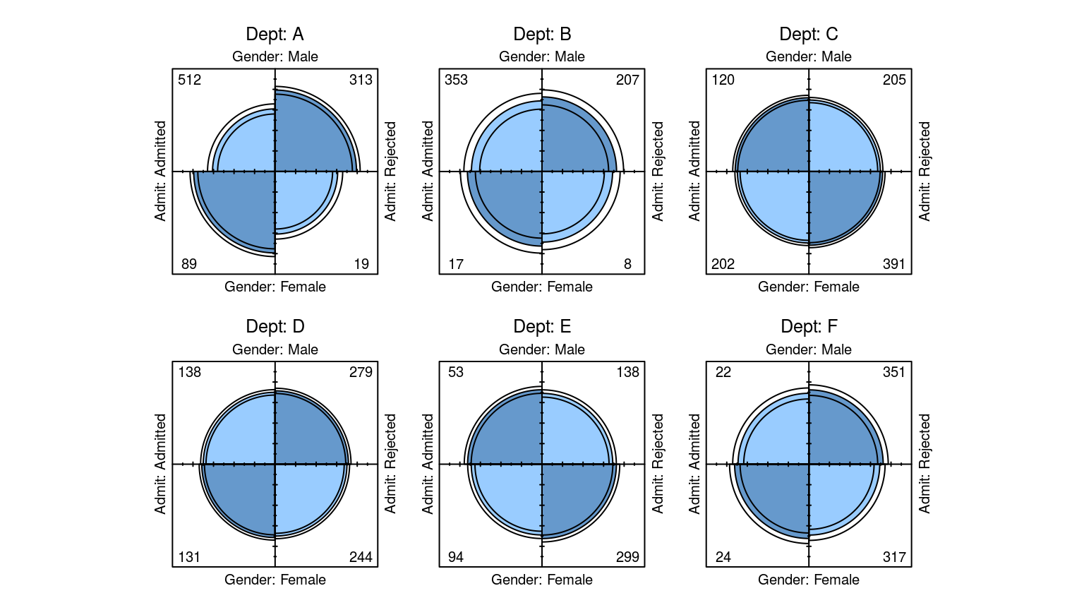
四折图 fourfoldplot

x <- aperm(UCBAdmissions, c(2, 1, 3))
fourfoldplot(x, mfcol=c(2, 3))

添加图形元素

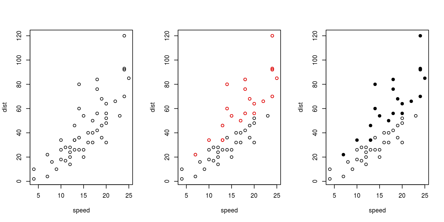
添加点 points

par(mfrow=c(1,3))
plot(cars)
plot(cars);points(cars[cars$dist > 2.6 * cars$speed,], col='red')
plot(cars);points(cars[cars$dist > 2.6 * cars$speed,], pch=19)

点型`pch`

pch代表点的种类，可以是整数

NA: 无符号
0:18: S兼容的矢量符号
19:25: R独特的矢量符号
32:127: ASCII字符，如33为感叹号
128:255: 本地符号
-32: … Unicode编码的点

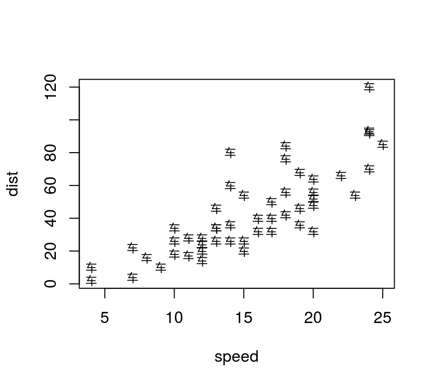
你甚至可以用其他文本符号

plot(cars, pch="\u8F66", cex=0.75)

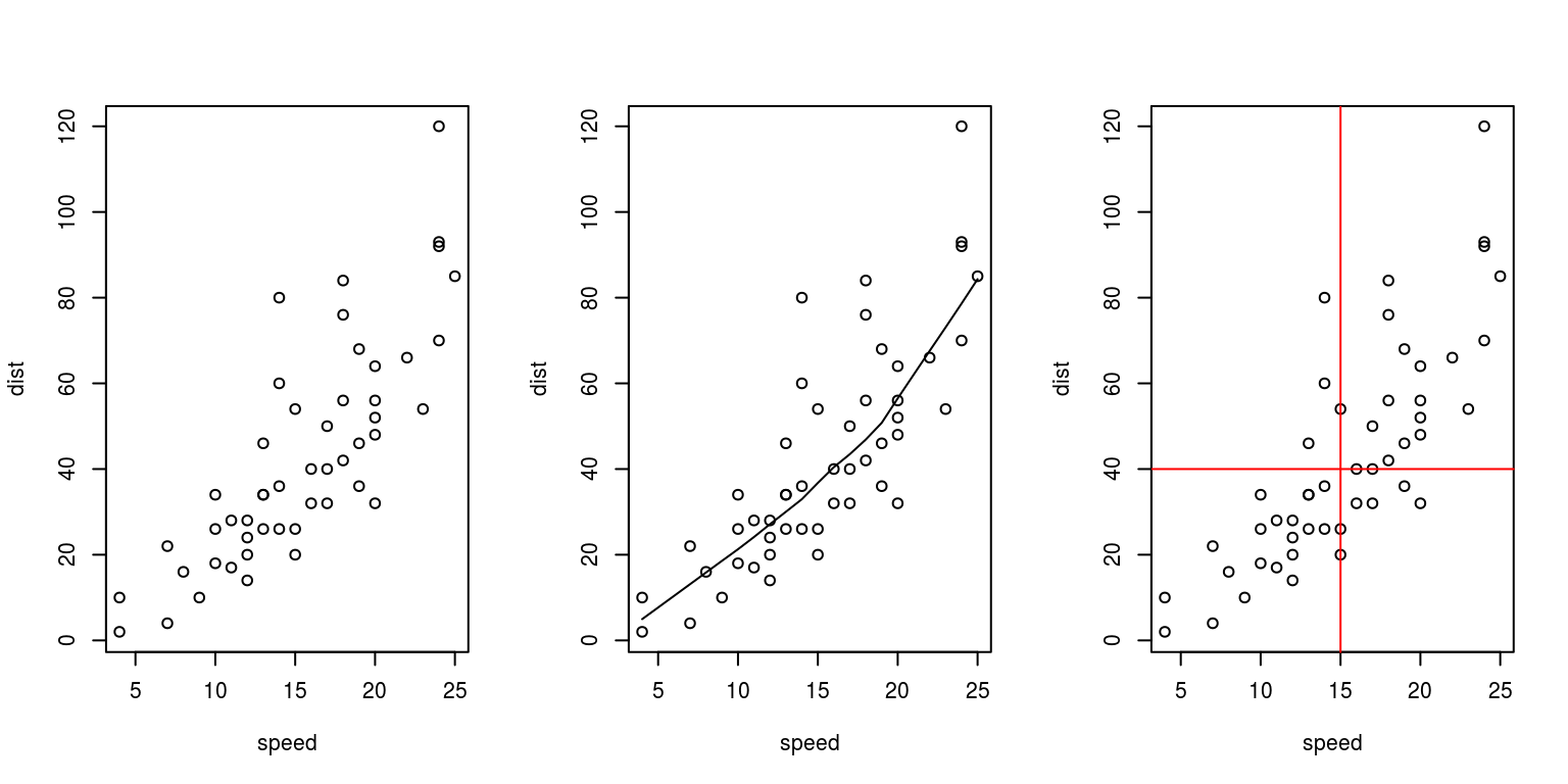
添加线条 lines

par(mfrow=c(1,3))
plot(cars)
plot(cars);lines(stats::lowess(cars))
plot(cars);abline(h=40,v=15,col="red")

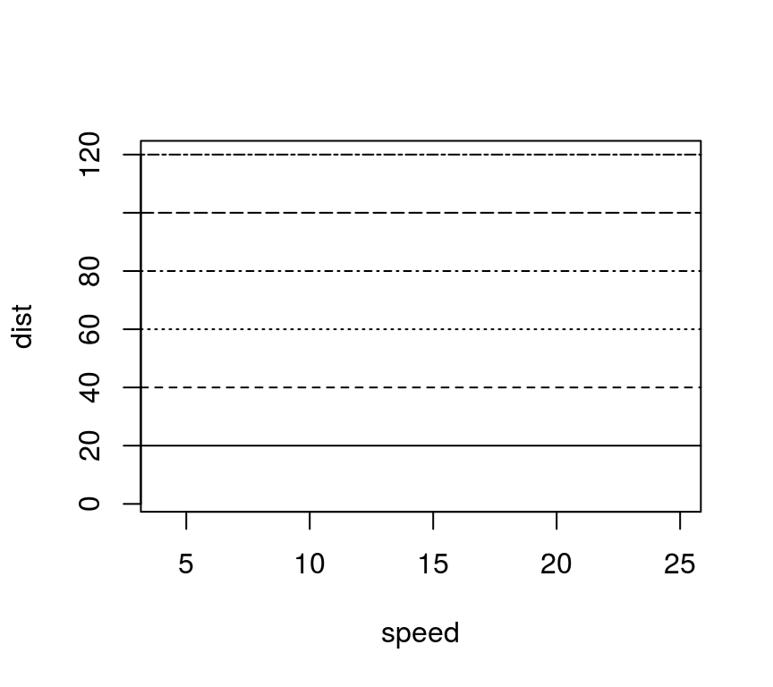
线型`lty`

lty是线条形状，可以是整数，或一个不超过8位的数值文本(连-断-连-断…的形式)

0 = 空白 blank
1 = 实线 solid(默认)
2 = 短划虚线 dashed，等价于"44"
3 = 点虚线 dotted，等价于"13"
4 = 点划虚线 dotdash，等价于"1343"
5 = 长划虚线 longdash，等价于"73"
6 = 双划虚线 twodash，等价于"2262"

plot(cars, type='n')
for (i in 1:6) abline(h=20*i, lty=i)

添加线段segments / 箭头arrows

x <- stats::runif(12); y <- stats::rnorm(12)
plot(x, y)
s <- seq(length(x)-1); s <- s[-length(s)]
segments(x[s], y[s], x[s+2], y[s+2], col= 'pink')

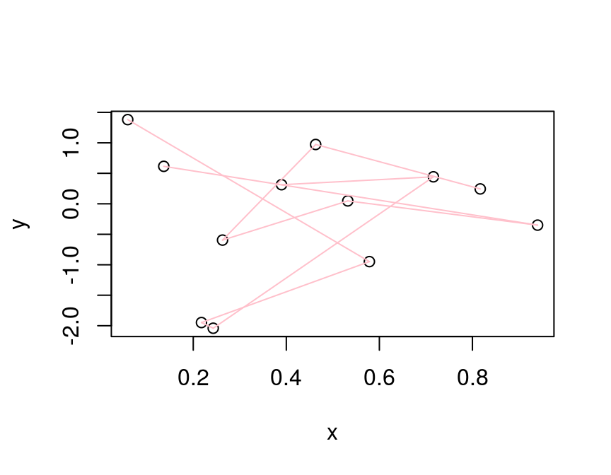
x <- stats::runif(12); y <- stats::rnorm(12)
plot(x, y)
s <- seq(length(x)-1)  # one shorter than data
arrows(x[s], y[s], x[s+1], y[s+1], col= 1:3)

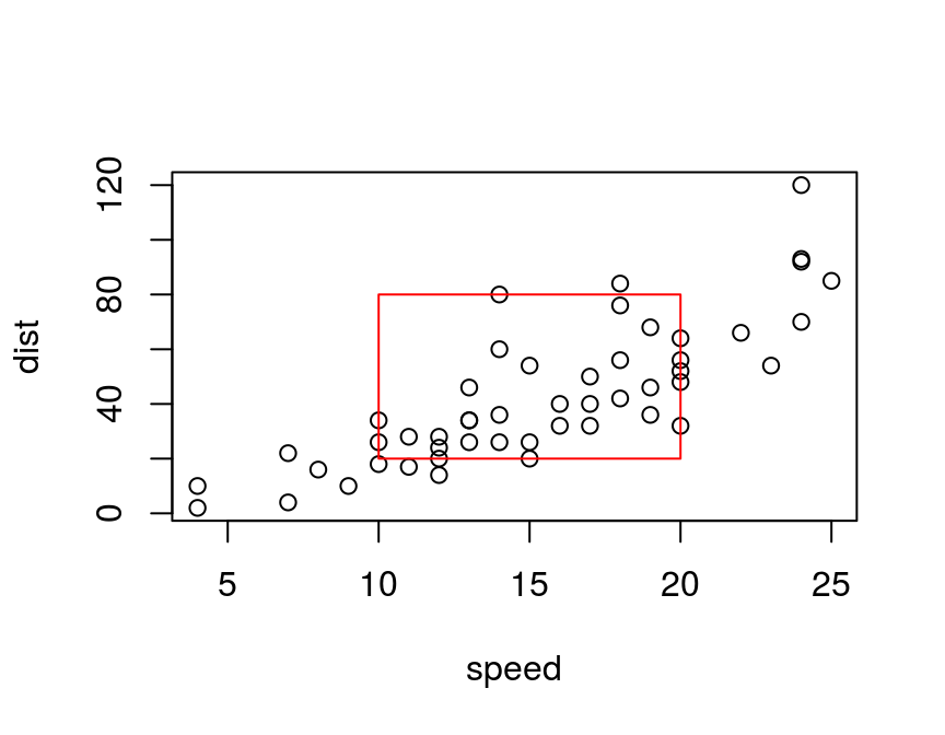
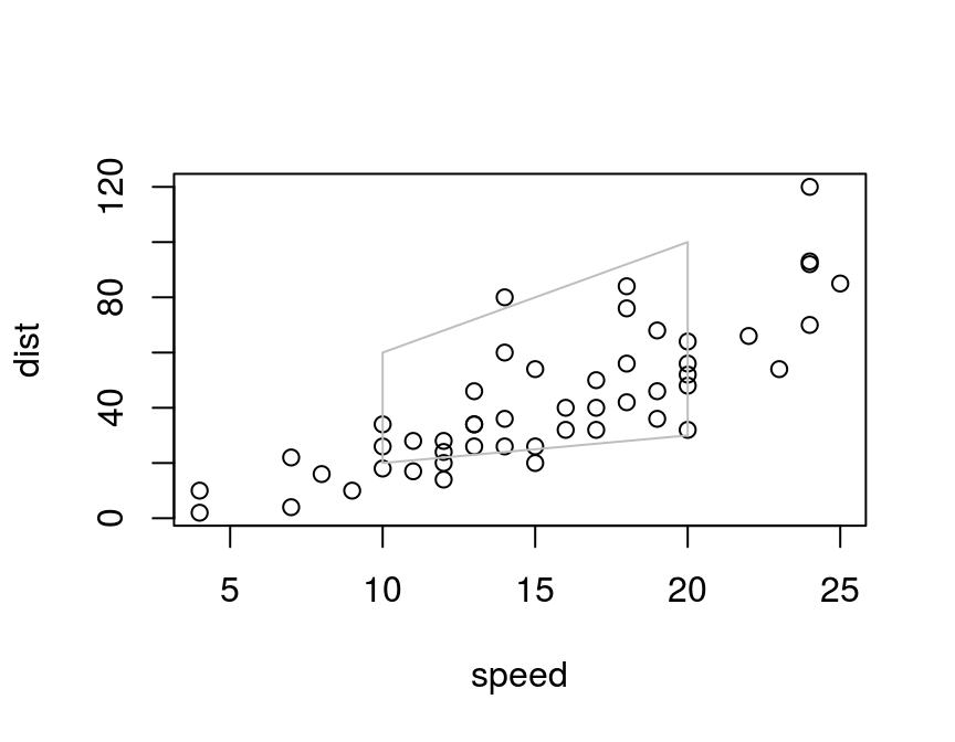
添加方块rect / 多边形 polygon

plot(cars)
rect(10, 20, 20, 80, border="red")

plot(cars)
polygon(c(10, 20, 20, 10), c(
    20, 30, 100, 60), border="gray")

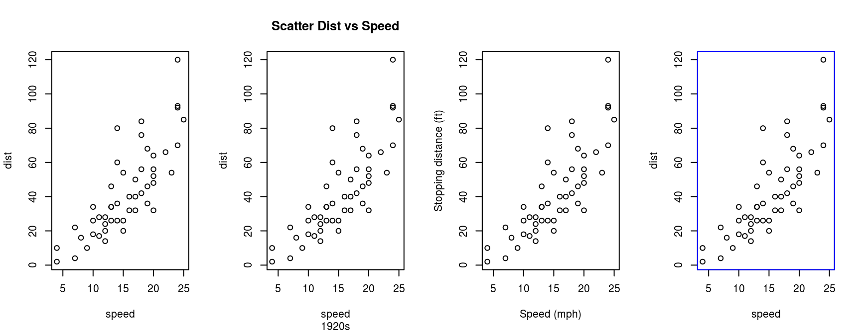
标注

标题 title、坐标轴 axis、边框 box

par(mfrow=c(1, 4))
plot(cars)
plot(cars); title("Scatter Dist vs Speed", sub="1920s")
plot(cars, xlab="Speed (mph)", ylab="Stopping distance (ft)")
plot(cars); box(col="blue")

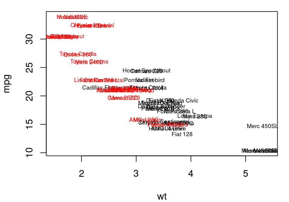
文字标注 text / 图例 legend

par(mar=c(4, 4, 1, 1))
with(mtcars, plot(wt, mpg, type="n"))  # 不出图
with(subset(mtcars, am==0), 
     text(wt, mpg, labels=row.names(mtcars),
     cex=0.6, col=1))
with(subset(mtcars, am==1), 
     text(wt, mpg, labels=row.names(mtcars),
     cex=0.6, col=2))

par(mar=c(4, 4, 1, 1))
with(mtcars, plot(wt, mpg), type='n')  # 不出图
with(subset(mtcars, am==0), 
     points(wt, mpg, pch=20, col=1))
with(subset(mtcars, am==1), 
     points(wt, mpg, pch=20, col=2))
legend("topright", pch=20, col=c(1, 2), 
       legend=c("Auto", "Manual"))

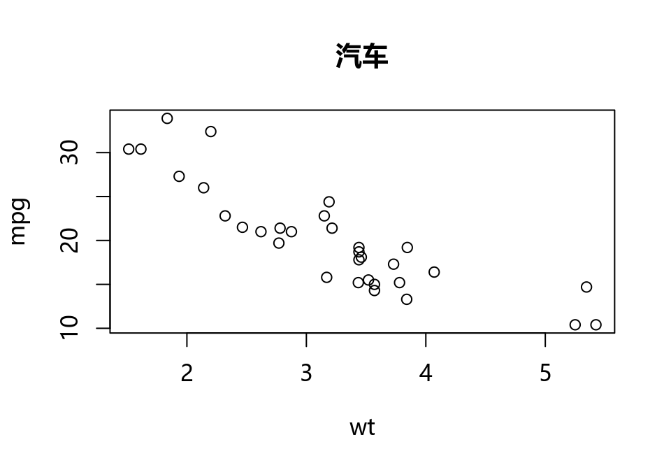
自定义字体: `extrafont`包

family参数可指定字体，但默认只支持"serif"、"sans"、"mono"等值
利用extrafont可将操作系统字体映射到R作图系统
使用方法
- install.packages("extrafont")
- extrafont::font_import()
- fonttable查看映射字体名称
- 使用fonttable()$FullName列表中的注册字体名称

library(extrafont)
with(mtcars, plot(wt, mpg, main='汽车', 
        family="Microsoft YaHei"))

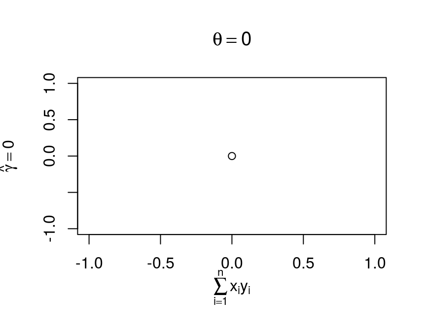
数学符号 (`?plotmath`)

expression()

plot(0, 0, main = expression(theta == 0),
     ylab = expression(hat(gamma) == 0),
     xlab = expression(sum(x[i] * y[i], i==1, n)))

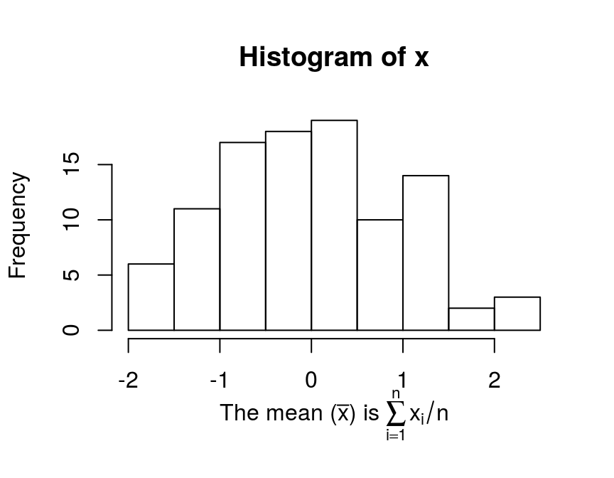
几部分文本拼接: *符号

x <- rnorm(100)
hist(x, xlab=expression(
  "The mean (" * bar(x) * ") is " * sum(x[i]/n,i==1,n)))

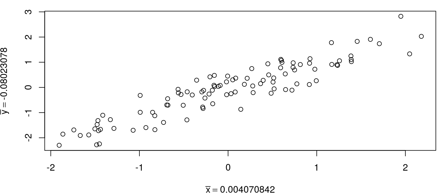
`substitute`函数

如果表达式中包含实时运算，要用substitute函数转义

par(mar=c(4, 4, 1, 1))
x <- rnorm(100)
y <- x + rnorm(100, sd = 0.5)
plot(x, y, xlab=substitute(bar(x) == k, list(k=mean(x))),
     ylab=substitute(bar(y) == k, list(k=mean(y))))

Thank you!

返回目录

目录