A03-05 ggplot2绘图系统

2017-05-20 16:30:23

作图流程

关于ggplot2

绘图语法Grammar of Graphics (by Leland Wilkinson)的程序实现
作者是 Hadley Wickham，R社区最知名的开发者之一
Grammar of Graphics的核心理念: 分层(layered grammar)
- 作图过程被抽象为一系列层的叠加
- 一幅图的元素 (名词)包括:
  - 数据data
  - 变量映射mapping
  - 图层layers
    - 几何形状geometric object, 统计转换statistic transforamtion, 位置偏移position adjustment, 美学映射aesthetic mapping
  - 尺度scale
  - 坐标coordinate system
  - 分面facet
- 针对各类元素，封装了丰富的处理函数(动词)
- GoG语法用统一的结构串联这些名词、动词，提供了一个处理图层的通用框架，兼备一致性和灵活性

流程

快速调用方法(类似lattice): `qplot()`

逐步调用方法

初始化 ggplot(): 初始化一个ggplot对象
绘制图层 geom_<形状>: geom_函数家族整合美学映射函数aes_、统计转换参数stat、位置偏移参数position、其他美学参数width、color等
修改尺度 scale_<尺度类型>: scale_函数家族用来指定视觉通道的映射方法
坐标系 coord_<坐标系>: coord_函数家族用来调整坐标系
分面 facet_grid/facet_wrap: 指定分面依据
美学修饰
- guides: 调整尺度和视觉通道的映射关系
- theme: 低级函数，修改图中每个部件的呈现形式
- ggtitle, xlab, ylab: 图/坐标轴标题
- annotate: 图上加注

快速调用

语法

qplot用来快速生成统计图，但自定义弹性不大

qplot(x, y = NULL, ..., data, facets = NULL, margins = FALSE,
  geom = "auto", xlim = c(NA, NA), ylim = c(NA, NA), log = "",
  main = NULL, xlab = deparse(substitute(x)),
  ylab = deparse(substitute(y)), asp = NA, stat = NULL, position = NULL)

x, y, …: 传入各个图层的变量
data: 数据源，一般是data.frame
facets, margins: 分面公式，是否显示边际分面
geom: 向量，呈现为哪种几何形状

Hello World

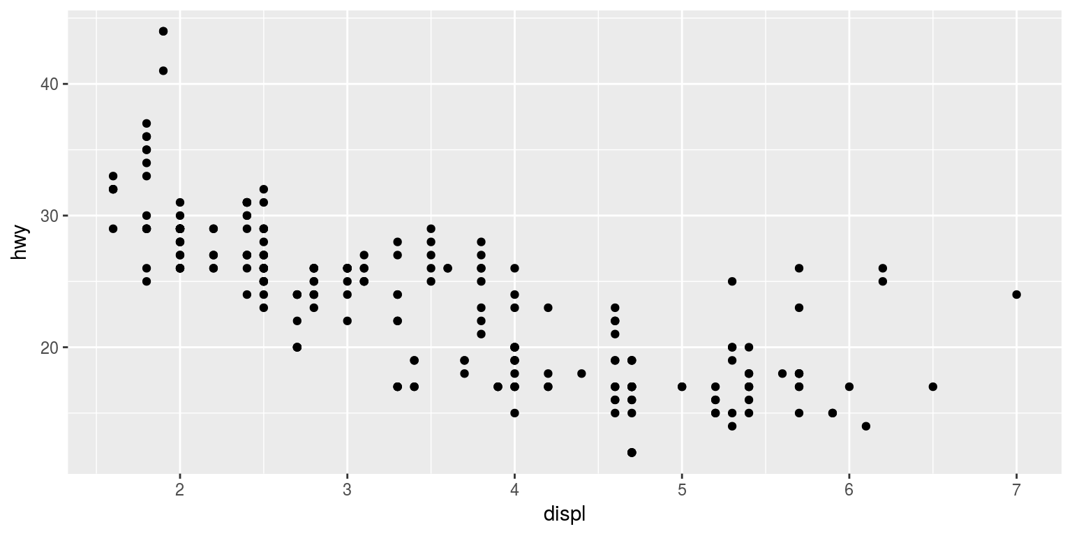
指定连续变量x,y，自动适配散点图

library(ggplot2)
qplot(displ, hwy, data = mpg)

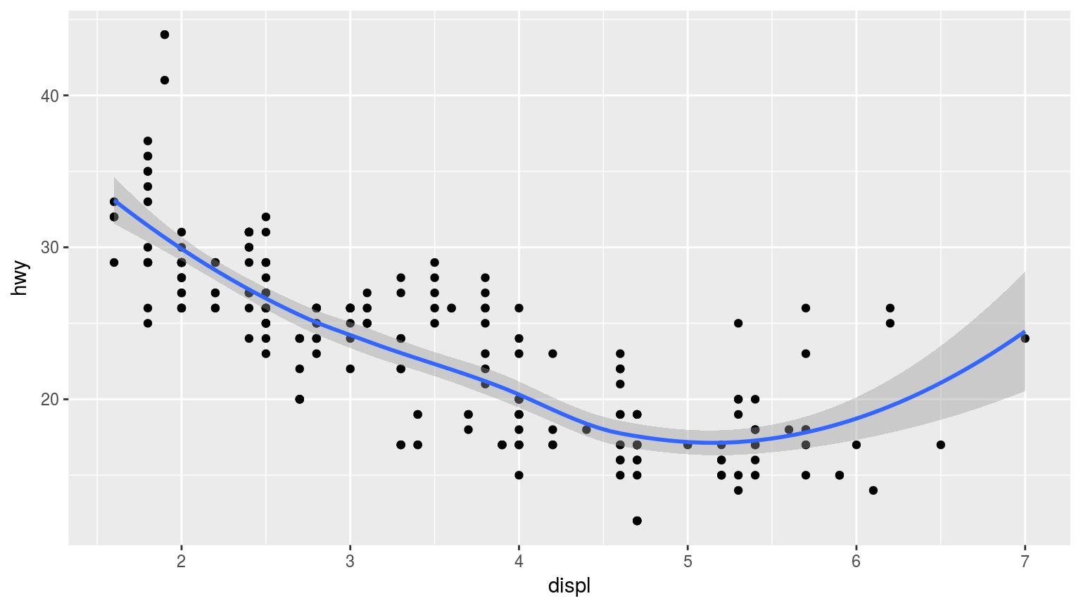
添加图层

qplot(displ, hwy, data = mpg, geom = c("point", "smooth"))

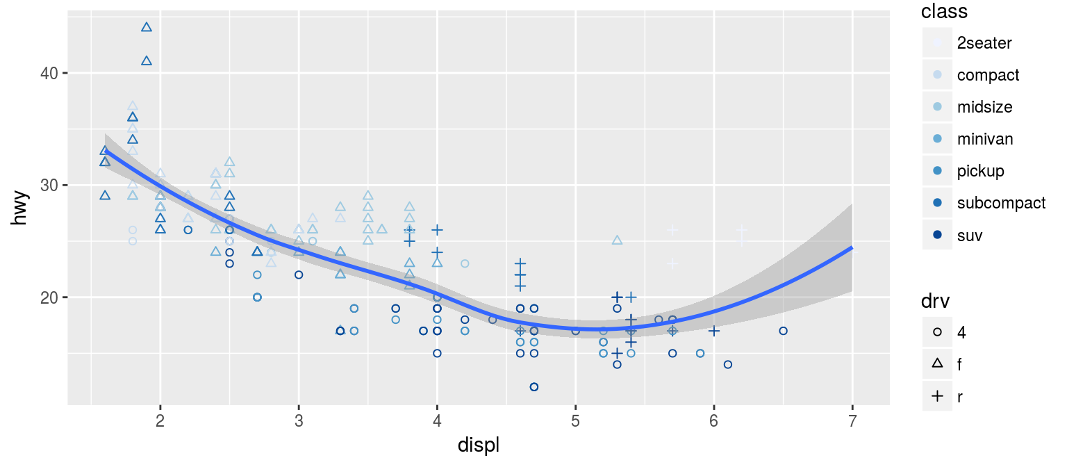
尺度映射

将class映射到颜色通道，drv映射到形状

qplot(displ, hwy, data = mpg, shape = drv, color = class)

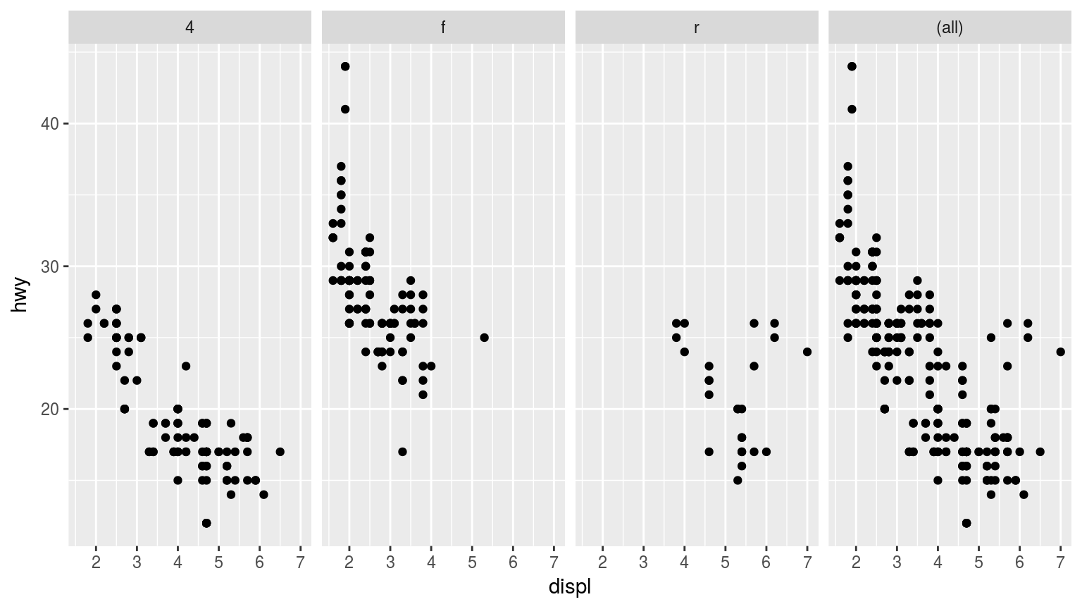
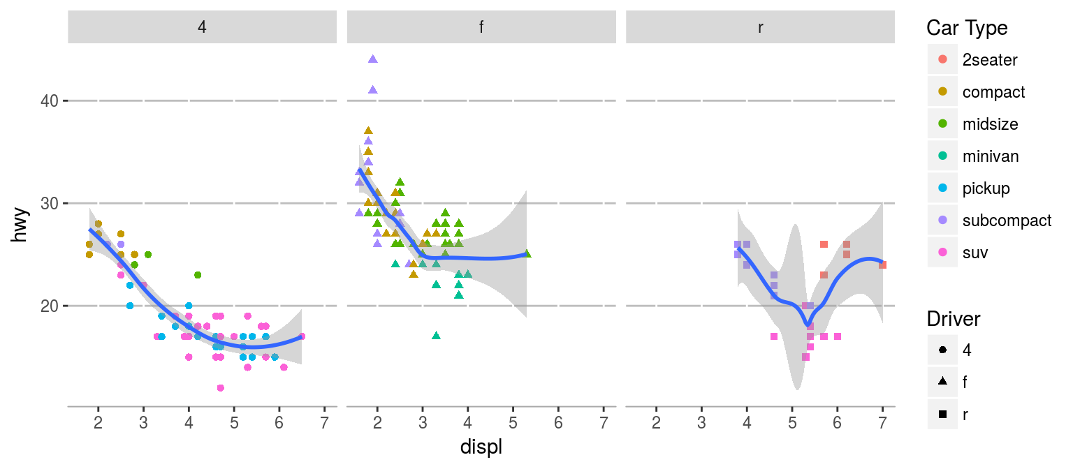
分面

qplot(displ, hwy, data = mpg, facets = . ~ drv, margins = TRUE)

逐步调用

初始化 (`ggplot`)

ggplot(data = NULL, mapping = aes(), ..., environment = parent.frame())

语法
- data: 源数据，如不是data.frame，会先被fortify函数预处理
- mapping: 美学映射，通过aes函数传入
三种主要调用形式:
1. ggplot(df, aes(x, y, <other aesthetics>))
2. ggplot(df)
3. ggplot(): 如果一幅图要用到多个独立的数据源，data可留空
初始化以后形成一个ggplot对象，但没有任何图层，因此不能显示

图层 (`geom_`)

geom_<形状>(mapping = NULL, data = NULL, stat, position, ..., na.rm = FALSE, 
    show.legend = NA, inherit.aes = TRUE)

mapping: 美学映射，可通过aes或aes_函数指定。一般inherit.aes为TRUE，即从初始化的ggplot对象直接继承美学映射参数。
data: 该图层用到的数据集
- NULL: 继承初始化的ggplot对象所包含的数据
- 一个data.frame或其他对象，将覆盖初始数据
- 一个function，该函数返回值必须是数据框
stat: 统计转换方法，如"density", "count"
position: 位置调整参数
- 文本，如"stack", "dodge"
- 函数，如position_stack, position_dodge
…: 通常是该图层的通用美学属性，如color, fill, 等
show.legend: 可以是NA、TRUE或FALSE

`aes` 美学/视觉通道映射: 映射谁?

aes(x, y, ...)

传入参数可以是变量名，也可以是函数计算式
常见的美学映射属性包括（各自适用于特定geom_）

- x: x轴/rho变量
- y: y轴/theta变量
- xmin: x最小值
- xmax: x最大值
- ymin: y最小值
- ymax: y最大值
- xend: x终点
- yend: y终点
- alpha: 透明度
- colour: 边线色

- fill: 填充色
- group: 分组
- linetype: 线型
- size: 粗细/大小
- xintercept: x截距
- yintercept: y截距
- slope: 斜率
- weight: 权重
- shape: 形状
- stroke: 描边
- map_id: 地图多变性id

尺度 (`scale_`): 怎么映射?

scale_<视觉通道>_<映射方法>(...)

视觉通道:
- x
- y
- colour
- fill
- alpha
- linetype
- radius
- shape
- size

映射方法:
- continuous/discrete: 连续/离散
- identity: 直接映射到视觉通道
- brewer/distiller: ColorBrewer色阶
- gradient/gradient2/gradientn: 渐变色阶
- date/datetime/time: 日期或时间
- grey/hue: 灰度/色谱
- log10/reverse/sqrt: 对数/逆序/开方
- manual: 手工指定(自定义)

坐标系 (`coord_`)

coord_cartesian: 直角平面坐标系
coord_fixed: 固定长宽比的直角坐标系
- coord_equal: 特例
coord_flip: 颠倒x/y
coord_map: 地图坐标系, projection指定投影方法
- coord_quickmap: 快捷地图坐标系
coord_polar: 极坐标系
coord_trans: 自定义调整坐标系

分面 (`facet_`)

在网格中定义矩阵分面
- facets必须是公式(行~列)

facet_grid(facets, margins = FALSE, scales = "fixed", space = "fixed",
  shrink = TRUE, labeller = "label_value", as.table = TRUE,
  switch = NULL, drop = TRUE)

把一维面板图转为二维
- facets可以是公式(~a + b,)或文本向量(c("a", "b"))

facet_wrap(facets, nrow = NULL, ncol = NULL, scales = "fixed",
  shrink = TRUE, labeller = "label_value", as.table = TRUE,
  switch = NULL, drop = TRUE, dir = "h", strip.position = "top")

修饰

`guides`调整尺度效果

guides可以在定义尺度时一并定义，也可单独用guides函数统一定义
实现同一效果:
- p + guides(colour = "colorbar", size = "legend", shape = "legend")
- p + guides(colour = guide_colorbar(), size = guide_legend(), shape = guide_legend())
- p + scale_colour_continuous(guide = "colorbar") + scale_size_discrete(guide = "legend") + scale_shape(guide = "legend")

`theme`调整图形部件

theme(line, rect, text, title, aspect.ratio, axis.title, axis.title.x,
  axis.title.x.top, axis.title.y, axis.title.y.right, axis.text, axis.text.x,
  axis.text.x.top, axis.text.y, axis.text.y.right, axis.ticks, axis.ticks.x,
  axis.ticks.y, axis.ticks.length, axis.line, axis.line.x, axis.line.y,
  legend.background, legend.margin, legend.spacing, legend.spacing.x,
  legend.spacing.y, legend.key, legend.key.size, legend.key.height,
  legend.key.width, legend.text, legend.text.align, legend.title,
  legend.title.align, legend.position, legend.direction, legend.justification,
  legend.box, legend.box.just, legend.box.margin, legend.box.background,
  legend.box.spacing, panel.background, panel.border, panel.spacing,
  panel.spacing.x, panel.spacing.y, panel.grid, panel.grid.major,
  panel.grid.minor, panel.grid.major.x, panel.grid.major.y, panel.grid.minor.x,
  panel.grid.minor.y, panel.ontop, plot.background, plot.title, plot.subtitle,
  plot.caption, plot.margin, strip.background, strip.placement, strip.text,
  strip.text.x, strip.text.y, strip.switch.pad.grid, strip.switch.pad.wrap, ...,
  complete = FALSE, validate = TRUE)

各部件可调用对应的element_函数进行编辑: element_line, element_rect, element_text

`theme_`套用主题

ggplot2中提供了一些主题函数，你也可以通过theme()自制主题
- theme_bw: 白底主题
- theme_classic: 经典主题
- theme_dark: 夜色主题
- theme_gray/theme_grey: (默认)灰色主题
- theme_light: 简洁主题
- theme_linedraw: 描线主题
- theme_minimal: 最小化主题
- theme_void: 极简主题
ggthemes包提供了包括更多主题，如excel, gdocs, economist, wsj

`ggtitle`, `xlab`, `ylab`定义标题

labs(...): 定义title, caption, subtitle及美学属性
xlab(label) / ylab(lable)/ ggtitle(label, subtitle = NULL)

`annotate`定义注释

annotate(geom, x = NULL, y = NULL, xmin = NULL, xmax = NULL,
  ymin = NULL, ymax = NULL, xend = NULL, yend = NULL, ...,
  na.rm = FALSE)

geom: 多边形类型，'text', 'rect', segment, pointrange
x, y, xmin, ymin, xmax, ymax, xend, yend: 在图中的位置，至少用到一个
…: 一般是美学属性

举例

同样的例子，用逐步法实现

p = ggplot(mpg, aes(displ, hwy))
p  # 仅初始化，什么都不显示

添加图层

将class映射到颜色通道，drv映射到形状

p = p + geom_point(aes(shape=drv, color=class)) + geom_smooth(method="loess")
p

尺度映射

调整映射方法

p1 = p + scale_shape_manual(values=c("4"=1, "f"=2, "r"=3)) + scale_color_brewer()
p1

分面

p = p + facet_grid(~drv)
p

套用主题

p + theme_light()

个性化修饰

p + theme(panel.background=element_blank(), panel.grid.major.y=element_line(color="gray"),
          axis.line.x=element_line(color="darkgray")) +
    guides(colour = guide_legend("Car Type", order=1), shape = guide_legend("Driver"))

一大堆用例

散点图 points

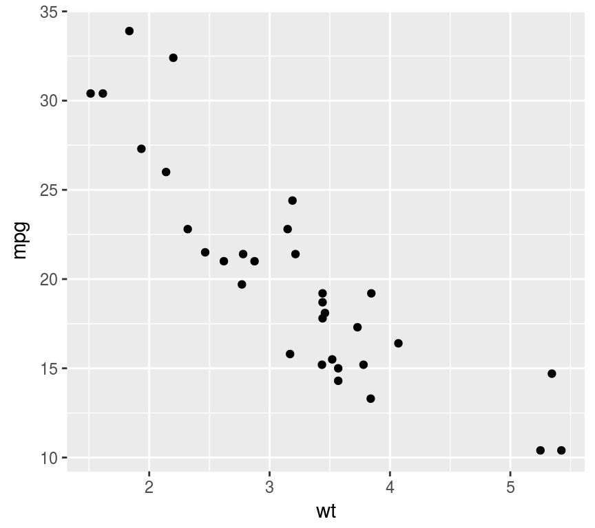
散点图: 两变量相关性

ggplot(mtcars, aes(wt, mpg)) + geom_point()

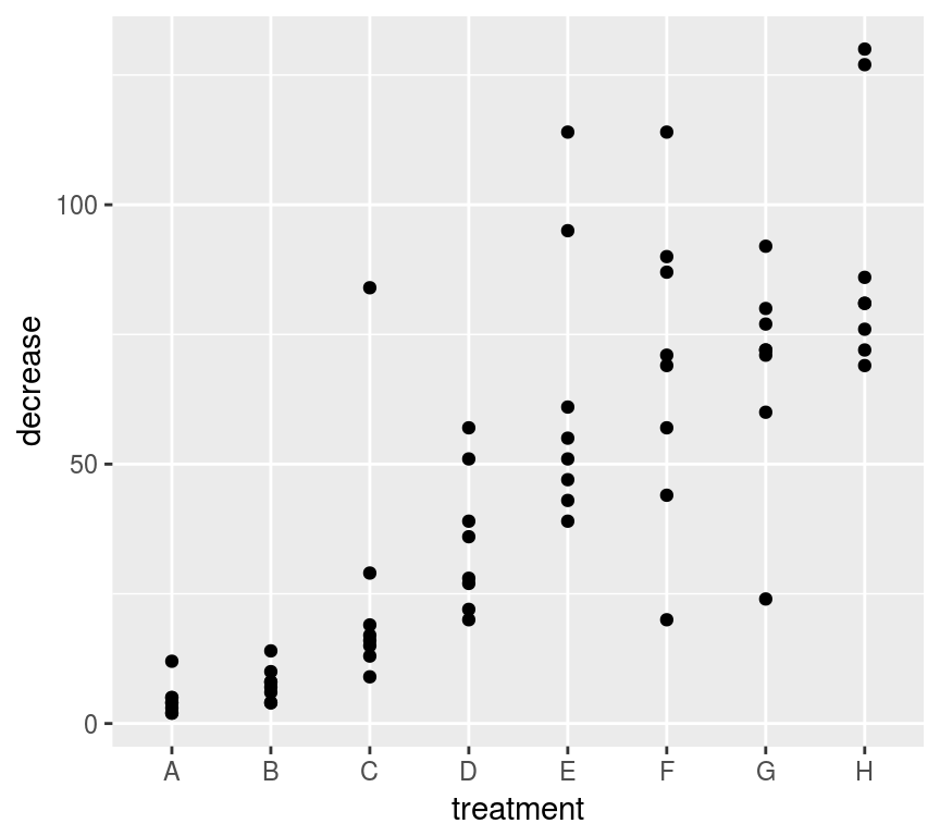
文本型变量作散点图

ggplot(OrchardSprays, aes(treatment, decrease)) + 
    geom_point()

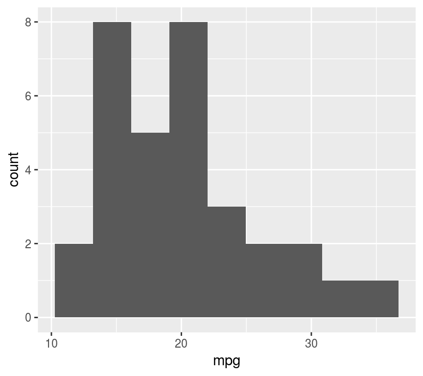
直方图 histogram

直方图: 单变量密度分布

ggplot(mtcars, aes(mpg)) + geom_histogram(bins=9)

或用密度图

ggplot(mtcars, aes(mpg)) + geom_density()

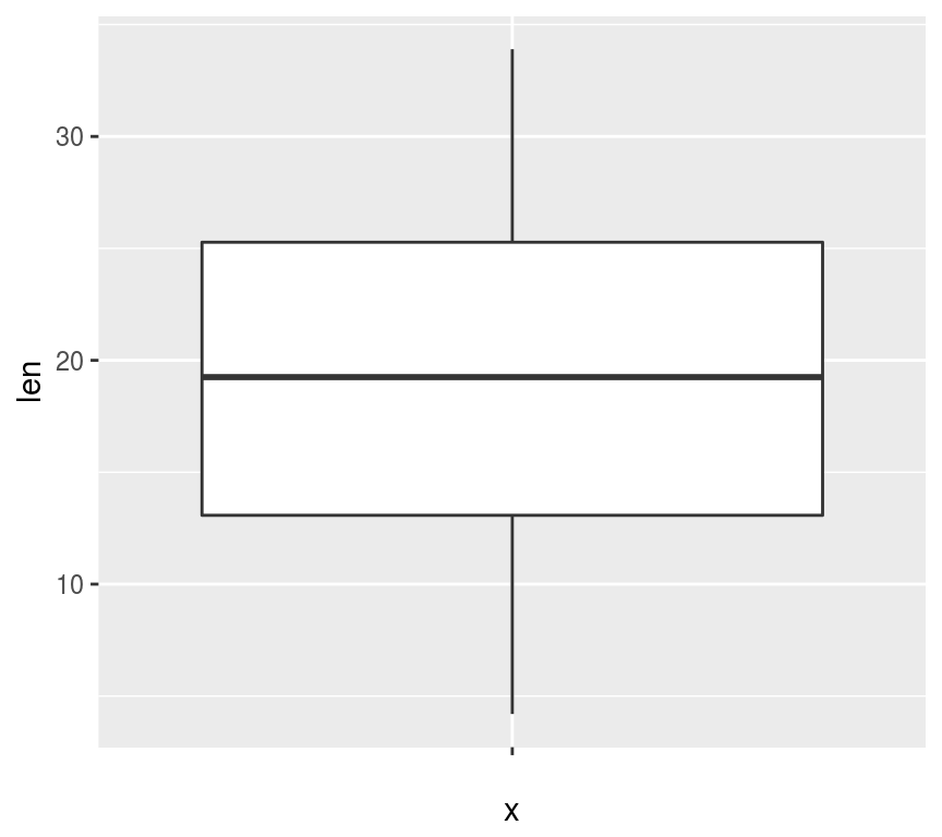
箱式图 boxplot

连续性变量的分布

ggplot(ToothGrowth, aes("", len)) + geom_boxplot()

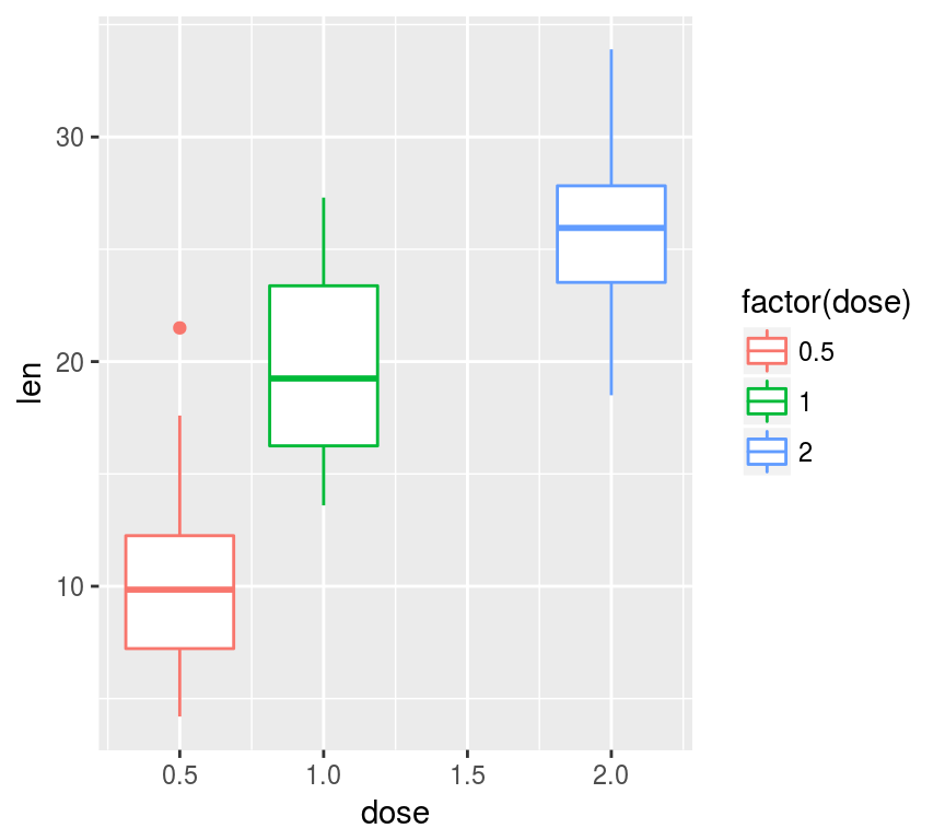
多个箱式图

ggplot(ToothGrowth, aes(dose, len, 
    color=factor(dose))) + geom_boxplot()

柱/条形图 barplot

分类变量的比较

hp <- data.frame(hp=mtcars$hp, 
                 names = row.names(mtcars))
ggplot(hp, aes(names, hp)) + geom_col()

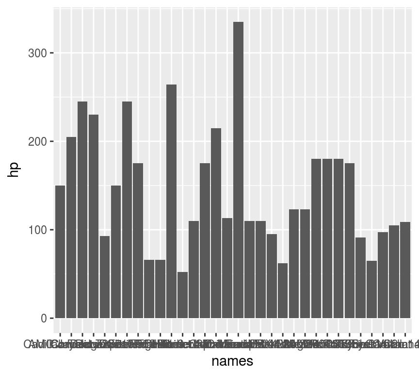
自变量较多时用横向条图

ggplot(hp, aes(names, hp)) + 
    geom_bar(stat="identity") + coord_flip()

折线图 lines

ts类型数据要先转换

AP <- data.frame(n=as.numeric(AirPassengers), 
                 t=zoo::as.Date(time(AirPassengers)))
ggplot(AP, aes(t, n)) + geom_line()

阶梯折线

ggplot(AP, aes(t, n)) + geom_step()

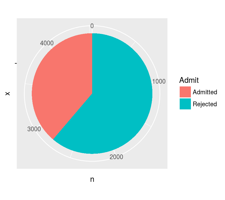
饼图 Pies

需要用coord_polar

admit <- data.frame(Admit=c("Admitted", "Rejected"), 
                    n=apply(UCBAdmissions, 1, sum))
ggplot(admit, aes("", n, fill=Admit)) + 
    geom_bar(stat="identity", position="stack", 
             width=1) + coord_polar(theta="y")

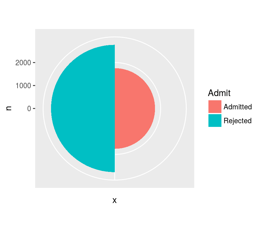
玫瑰图: position='dodge'

ggplot(admit, aes("", n, fill=Admit)) + 
    geom_bar(stat="identity", position="dodge", 
             width=1) + coord_polar()

Thank you!

返回目录

目录

作图流程

关于ggplot2

流程

快速调用方法(类似lattice): qplot()

逐步调用方法

快速调用

语法

Hello World

添加图层

尺度映射

分面

逐步调用

初始化 (ggplot)

图层 (geom_)

aes 美学/视觉通道映射: 映射谁?

尺度 (scale_): 怎么映射?

坐标系 (coord_)

分面 (facet_)

修饰

guides调整尺度效果

theme调整图形部件

theme_套用主题

ggtitle, xlab, ylab定义标题

annotate定义注释

举例

添加图层

尺度映射

分面

套用主题

个性化修饰

一大堆用例

散点图 points

直方图 histogram

箱式图 boxplot

柱/条形图 barplot

折线图 lines

饼图 Pies

快速调用方法(类似lattice): `qplot()`

初始化 (`ggplot`)

图层 (`geom_`)

`aes` 美学/视觉通道映射: 映射谁?

尺度 (`scale_`): 怎么映射?

坐标系 (`coord_`)

分面 (`facet_`)

`guides`调整尺度效果

`theme`调整图形部件

`theme_`套用主题

`ggtitle`, `xlab`, `ylab`定义标题

`annotate`定义注释