A04-06 时间序列分析

2017-05-18 21:04:52

数据结构

`ts`、`xts`、`zoo`类

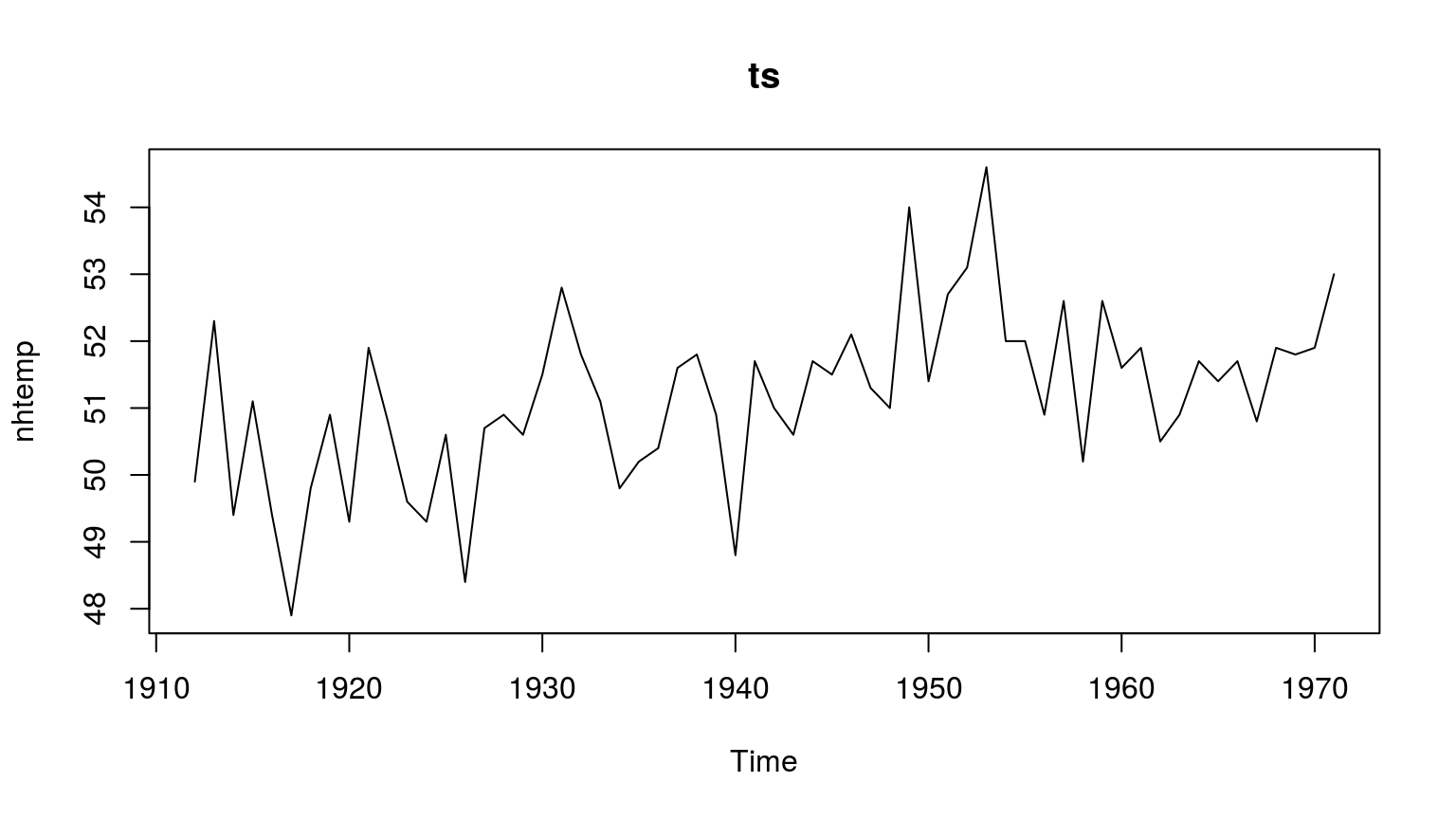
stats内置的ts类

> str(nhtemp)
 Time-Series [1:60] from 1912 to 1971: 49.9 52.3 49.4 51.1 49.4 47.9 ...

xts包的xts类

> str(as.xts(nhtemp))
An ‘xts’ object on 1912-01-01/1971-01-01 containing:
  Data: num [1:60, 1] 49.9 52.3 49.4 51.1 49.4 47.9 49.8 50.9 49.3 51.9 ...
  Indexed by objects of class: [Date] TZ: UTC
  xts Attributes:  
 NULL

zoo包的zoo类

> str(as.zoo(nhtemp))
‘zooreg’ series from 1912 to 1971
  Data: num [1:60] 49.9 52.3 49.4 51.1 49.4 47.9 49.8 50.9 49.3 51.9 ...
  Index:  num [1:60] 1912 1913 1914 1915 1916 ...
  Frequency: 1

定距时间序列

ts(data = NA, start = 1, end = numeric(), frequency = 1,
   deltat = 1, ts.eps = getOption("ts.eps"), class = , names = )

frequency: 12(月), 4(季度), 1(年)
start/end: 起止时间

> ts(1:21, freq=12, start=1990)
     Jan Feb Mar Apr May Jun Jul Aug Sep Oct Nov Dec
1990   1   2   3   4   5   6   7   8   9  10  11  12
1991  13  14  15  16  17  18  19  20  21  

> ts(1:7, freq=4, start=c(1990, 2))
     Qtr1 Qtr2 Qtr3 Qtr4
1990         1    2    3
1991    4    5    6    7

不规则时间序列

xts(x = NULL, order.by = index(x), frequency = NULL, unique = TRUE,
    tzone = Sys.getenv("TZ"), ...)

order.by: 时间/日期向量
frequency: order.by的频率

> xts(1:5, order.by=as.Date("1990-1-1")+c(0,3,5,11,12))
           [,1]
1990-01-01    1
1990-01-04    2
1990-01-06    3
1990-01-12    4
1990-01-13    5

可视化

时间序列图: `plot.ts`

invisible(Sys.setlocale("LC_TIME", "C"))
plot(nhtemp, main="ts")

时间序列图: `plot.xts`

library(xts)
plot(xts(1:21, order.by=as.Date("1990-1-1")+cumsum(rep(c(1,3,7,11:14), 3))), main="xts")

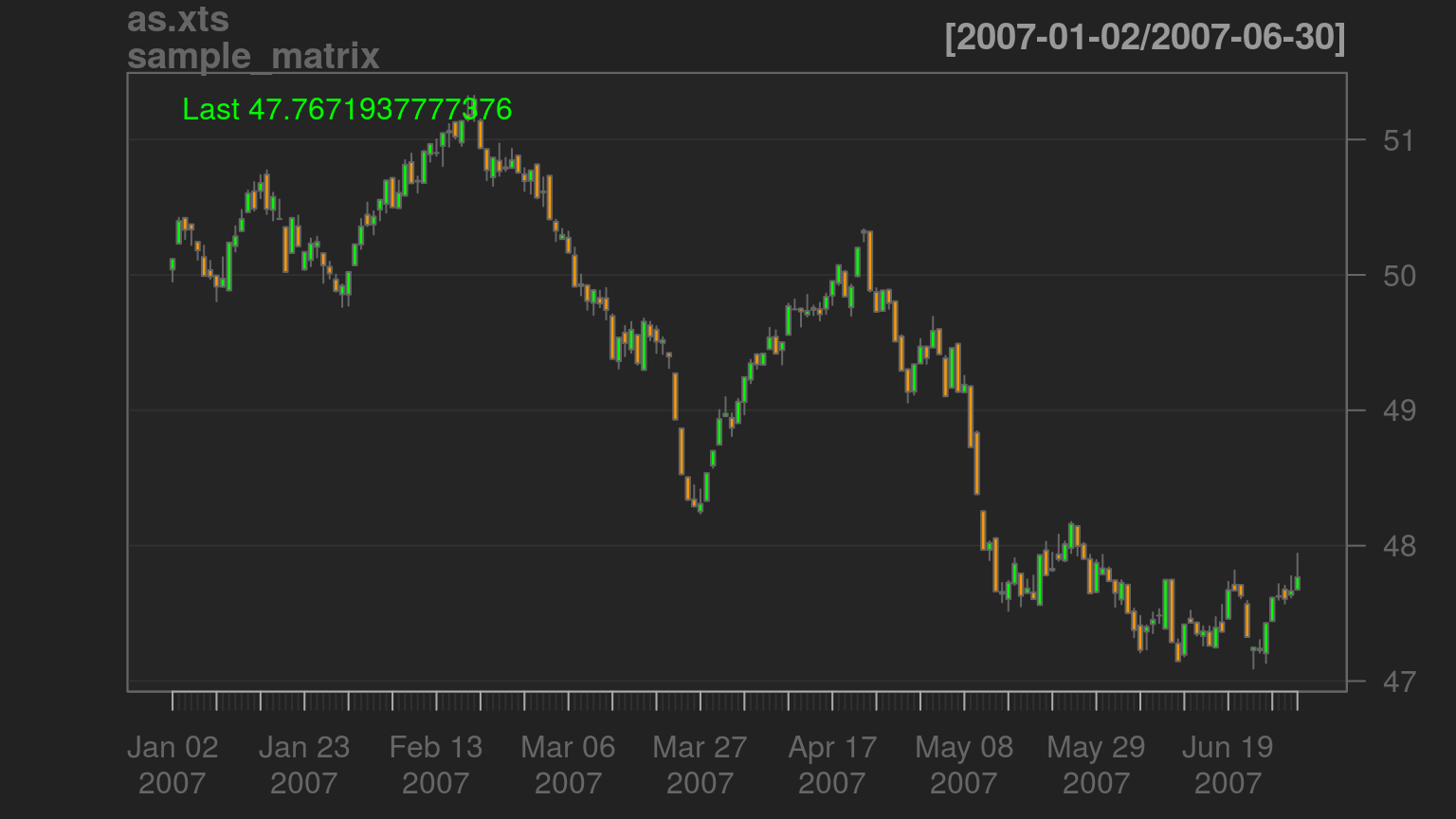
时间序列图: `quantmod`包

library(quantmod); data(sample_matrix)
chartSeries(as.xts(sample_matrix))

时间序列图: `dygraphs`包

library(dygraphs)
dyCandlestick(dygraph(sample_matrix))

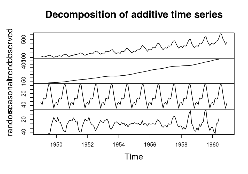
分解时间序列 Decomposition

季节性和非季节数据

季节性数据包括3种成分的变异: 趋势性、季节性、不规则部分

plot(as.xts(AirPassengers))

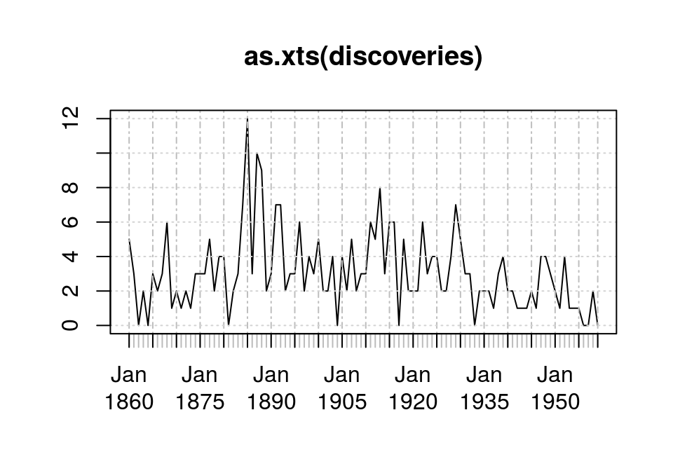
非季节性数据包括2种成分的变异: 趋势性、不规则部分

plot(as.xts(discoveries))

季节性数据(1) - `decompose`移动平均法

3个成分: trend, seasonal, random

相加模型

plot(decompose(AirPassengers))

相乘模型

plot(decompose(AirPassengers, type="multiplicative"))

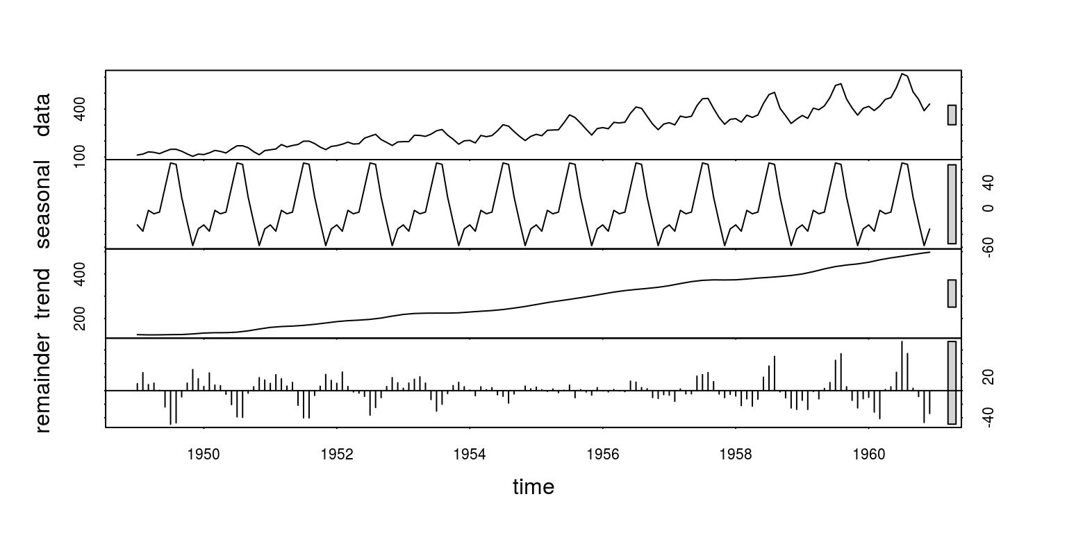
季节性数据(2) - 局部加权回归法`STL`

3个成分: seasonal, trend, remainder

plot(stl(AirPassengers, s.window="periodic"))

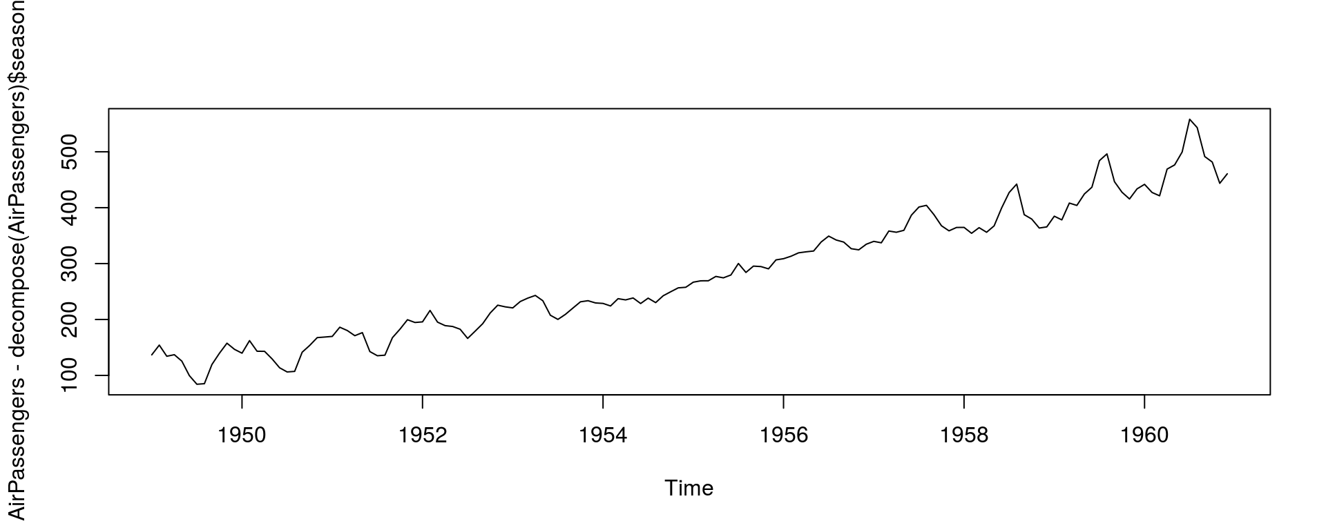
季节性数据(3) - 调整

调整不关注的变异因素(如调整季节因素seasonal)

plot(AirPassengers - decompose(AirPassengers)$seasonal)

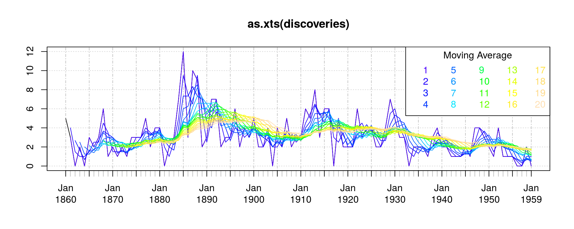
非季节性数据

平滑法(TTR::SMA)移动时间序列

library(TTR); library(xts)
plot(as.xts(discoveries))
for (i in 1:20) lines(as.xts(SMA(discoveries, n=i)), col=topo.colors(20)[i])
legend("topright", legend=1:20, text.col=topo.colors(20), ncol=5, title="Moving Average", title.col="black")

指数平滑法
(Exponential Smoothing)

适用条件

用于描述时间序列数据和作短期预测，并不试图解释和理解成因。

指数平滑法计算出的预测区间，其预测误差必须是不相关的，且服从零均值、方差不变的正态分布

语法: HoltWinters(x, alpha=NULL, beta=NULL, gamma=NULL, ...)

指数平滑法	数据模型	趋势	季节变动	alpha	beta	gamma
简单指数平滑法	相加模型	恒定水平	没有季节性	0-1	FALSE	FALSE
Holt指数平滑法	可描述为相加模型	增长或降低趋势	没有季节性	0-1	0-1	FALSE
Holt-Winters指数平滑法	可描述为相加模型	增长或降低趋势	存在季节性	0-1	0-1	0-1

简单指数平滑法(1)

[1] 是否满足要求

plot(as.xts(Nile))

[2] HoltWinters

> HoltWinters(Nile, beta=FALSE, gamma=FALSE)

Holt-Winters exponential smoothing without 
    trend and without seasonal component.
Call:
HoltWinters(x = Nile, beta = FALSE, gamma = FALSE)

Smoothing parameters:
 alpha: 0.2465579
 beta : FALSE
 gamma: FALSE
 
Coefficients:
      [,1]
a 805.0389

alpha越接近0，则近期数据对预测的贡献越小

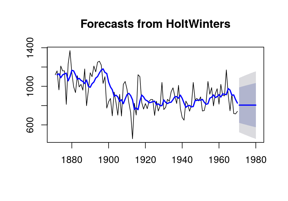
简单指数平滑法(2)

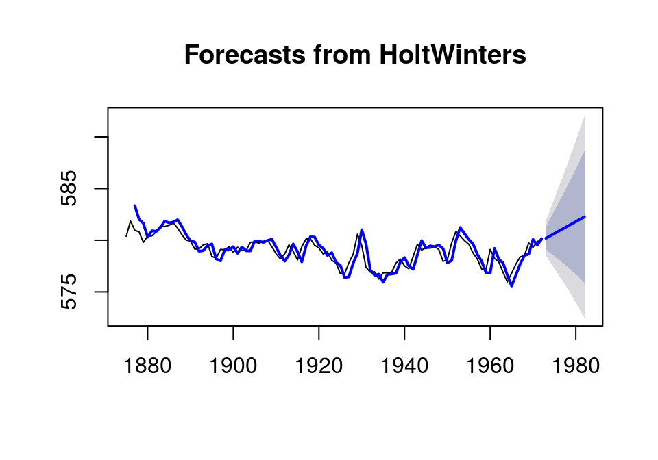
[3] 预测

library(forecast)
hw <- HoltWinters(Nile, beta=F, gamma=F)
forec <- forecast(hw, h=10); plot(forec)
lines(hw$fitted[,1], col='blue', lwd=2)

[4] 自相关检验及Ljung-Box检验

acf(forec$residuals, lag.max=20, na=na.pass)

> Box.test(forec$residuals, lag=20, type="Ljung-Box")
...
X-squared = 15.619, df = 20, p-value = 0.74

p值>0.05，不足以判定样本内预测误差在滞后1-20阶时是非零自相关的。(可认为不规则部分是白噪声)

简单指数平滑法(3)

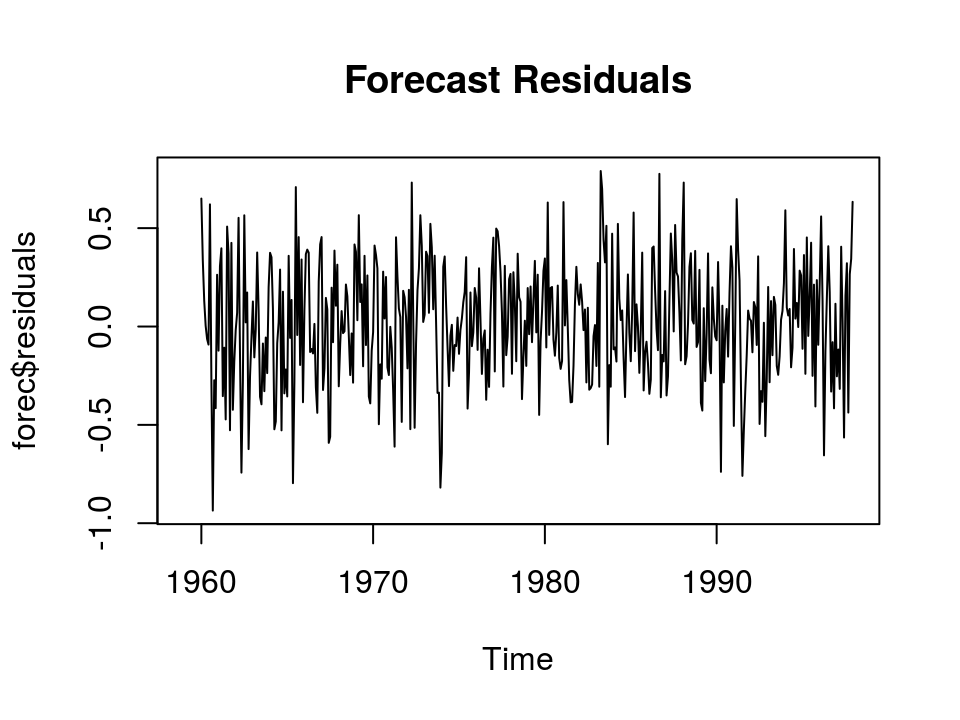
[5] 预测误差诊断

hist(forec$residuals, freq=FALSE)
lines(density(forec$residuals, na.rm=T), lwd=2)

预测误差大体服从零均值正态分布，但前期波动较后期大(方差有变化)。模型可能仍有改良空间。

plot(forec$residuals, main="Forecast Residuals")

Holt指数平滑法(1)

[1] 是否满足要求

plot(as.xts(LakeHuron))

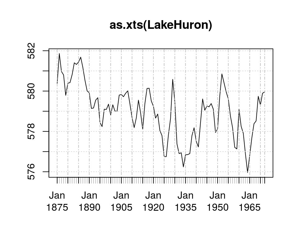
[2] HoltWinters

> HoltWinters(LakeHuron, gamma=FALSE)

Holt-Winters exponential smoothing with 
    trend and without seasonal component.

Call:
HoltWinters(x = LakeHuron, gamma = FALSE)

Smoothing parameters:
 alpha: 1
 beta : 0.1793351
 gamma: FALSE

Coefficients:
         [,1]
a 579.9600000
b   0.2300602

Holt指数平滑法(2)

[3] 预测

hw <- HoltWinters(LakeHuron, gamma=FALSE)
forec <- forecast(hw, h=10); plot(forec)
lines(hw$fitted[,1], col='blue', lwd=2)

[4] 自相关检验及Ljung-Box检验

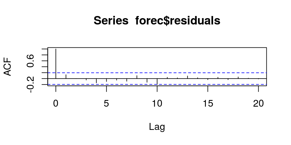
acf(forec$residuals, lag.max=20, na=na.pass)

> Box.test(forec$residuals, lag=20, type="Ljung-Box")
...
X-squared = 22.581, df = 20, p-value = 0.3098

p值>0.05，不足以判定样本内预测误差在滞后1-20阶时是非零自相关的。(可认为不规则部分是白噪声)

Holt指数平滑法(3)

[5] 预测误差诊断

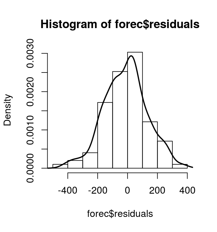
hist(forec$residuals, freq=FALSE)
lines(density(forec$residuals, na.rm=T), lwd=2)

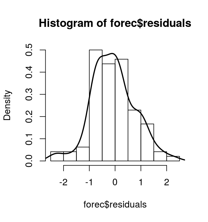
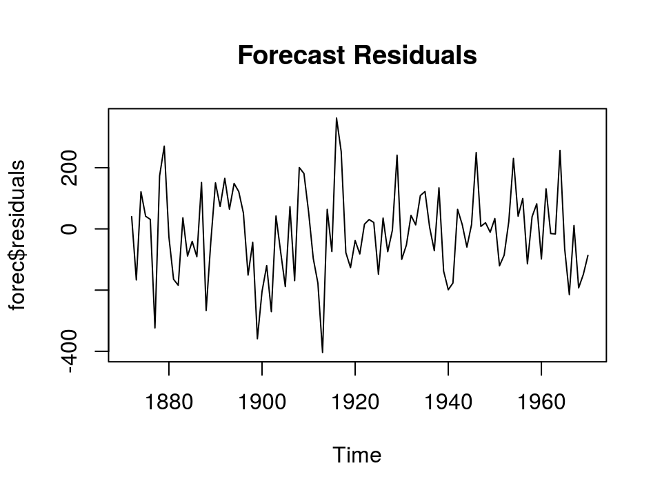
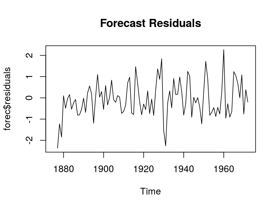
预测误差大体服从零均值正态分布，方差前后也大体无变化。模型可不用再改良。

plot(forec$residuals, main="Forecast Residuals")

Holt-Winters指数平滑法(1)

[1] 是否满足要求

plot(as.xts(co2))

[2] HoltWinters

> HoltWinters(co2)

Smoothing parameters:
 alpha: 0.5126484
 beta : 0.009497669
 gamma: 0.4728868

Coefficients:
           [,1]
a   364.7616237
b     0.1247438
s1    0.2215275
s2    0.9552801
s3    1.5984744
s4    2.8758029
s5    3.2820088
s6    2.4406990
s7    0.8969433
s8   -1.3796428
s9   -3.4112376
s10  -3.2570163
s11  -1.9134850
s12  -0.5844250

Holt-Winters指数平滑法(2)

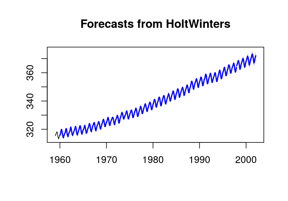
[3] 预测

hw <- HoltWinters(co2)
forec <- forecast(hw, h=50); plot(forec)
lines(hw$fitted[,1], col='blue', lwd=2)

[4] 自相关检验及Ljung-Box检验

acf(forec$residuals, lag.max=20, na=na.pass)

> Box.test(forec$residuals, lag=20, type="Ljung-Box")
...
X-squared = 25.896, df = 20, p-value = 0.1693

p值>0.05，不足以判定样本内预测误差在滞后1-20阶时是非零自相关的。(可认为不规则部分是白噪声)

Holt-Winters指数平滑法(3)

[5] 预测误差诊断

hist(forec$residuals, freq=FALSE)
lines(density(forec$residuals, na.rm=T), lwd=2)

预测误差大体服从零均值正态分布，方差前后也大体无变化。模型可不用再改良。

plot(forec$residuals, main="Forecast Residuals")

ARIMA模型

整合移动平均自回归(ARIMA)模型

ARIMA是时序分析中最常用的经典方法。它包含一个确定（explicit）的统计模型用于处理时间序列的不规则部分，而且允许不规则部分自相关。

通常先差分，把长期趋势、固定周期等信息提取出来，将非平稳序列变为平稳(stationary)序列后进行分析。剩余部分等价于一个ARMA(p,q)模型：

如不平稳，diff差分， ARIMA(p, d, q) ==> ARMA(p, q)
acf自回归图，判定q系数
pacf偏自回归图，判定p阶数
拟合arima(p, d, q)模型并预测
1. 如有季节性，选取合理的 arima(p, d, q)(P, D, Q)_m 模型
检验模型残差

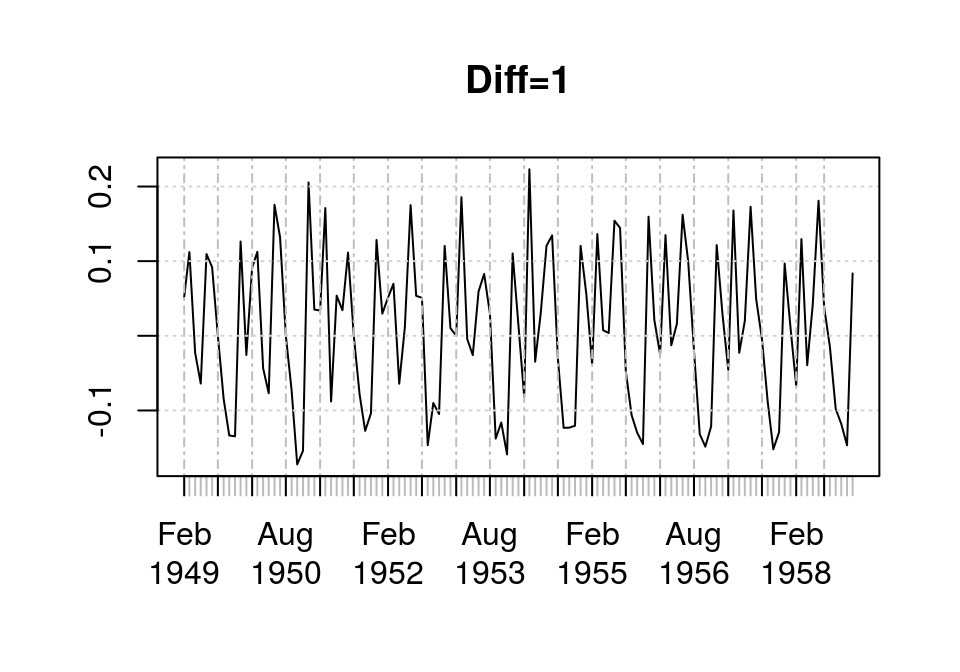
差分及增强的Dickey-Fuller单位根检验

library(forecast)
ap <- log(tsclean(AirPassengers))
ap1 <- ts(ap[1:120], start=c(1949,1), freq=12)
plot(as.xts(diff(ap1, 1)), main="Diff=1")

ADF平稳性检验

> library(tseries)
> adf.test(diff(ap1, 1), k=0)

    Augmented Dickey-Fuller Test

data:  diff(ap1, 1)
Dickey-Fuller = -9.1113, Lag order = 0, p-value = 0.01
alternative hypothesis: stationary

1阶差分后，AirPassengers数据(去掉季节趋势)可认为是平稳的

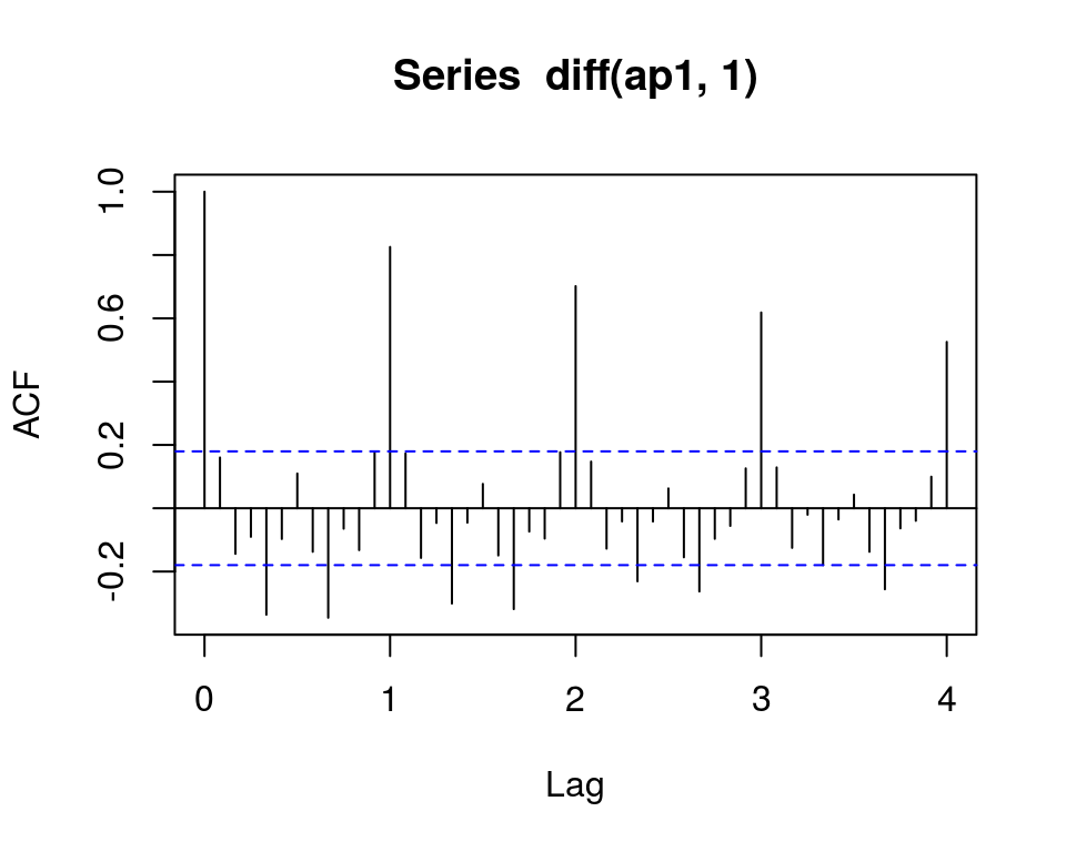
自回归图及偏自回归图

ACF: 滞后1阶起，自相关值即截尾 -> q=0或1

acf(diff(ap1, 1), lag.max=48)

PACF: 滞后1阶起，偏自相关值即截尾 -> p=0

pacf(diff(ap1, 1), lag.max=48)

构建Arima模型

Arima(p, d, q)(P, D, Q)_m模型选择原则

AIC或BIC尽可能小
参数尽可能少(尽可能简单)
可参考auto.arima

(P, D, Q)_m季节性参数的确定

分解时序观察到周期为12的季节性 -> D=1, m=12
差分后ACF图仍有周期为12的季节性 -> Q=1, m=12
差分后PACF图没有显示出明显的周期性 -> P=0

> m1 <- auto.arima(ap1); m1

Series: ap1 
ARIMA(0,1,1)(0,1,1)[12]            
Coefficients:
          ma1     sma1
      -0.3674  -0.5686
s.e.   0.1012   0.0892

sigma^2 estimated as 0.001384:  
    log likelihood=199.07
AIC=-392.14   AICc=-391.9   BIC=-384.12

> m2 <- Arima(ap1, order=c(0, 1, 0), 
+ seasonal=list(order=c(0, 1, 1), freq=12))
> m3 <- Arima(ap1, order=c(0, 1, 1), 
+ seasonal=list(order=c(0, 1, 2), freq=12))
> sapply(list(m1, m2, m3), function(x) {
+ x[c('aic','bic')]})

    [,1]      [,2]      [,3]     
aic -392.1358 -382.356  -390.1689
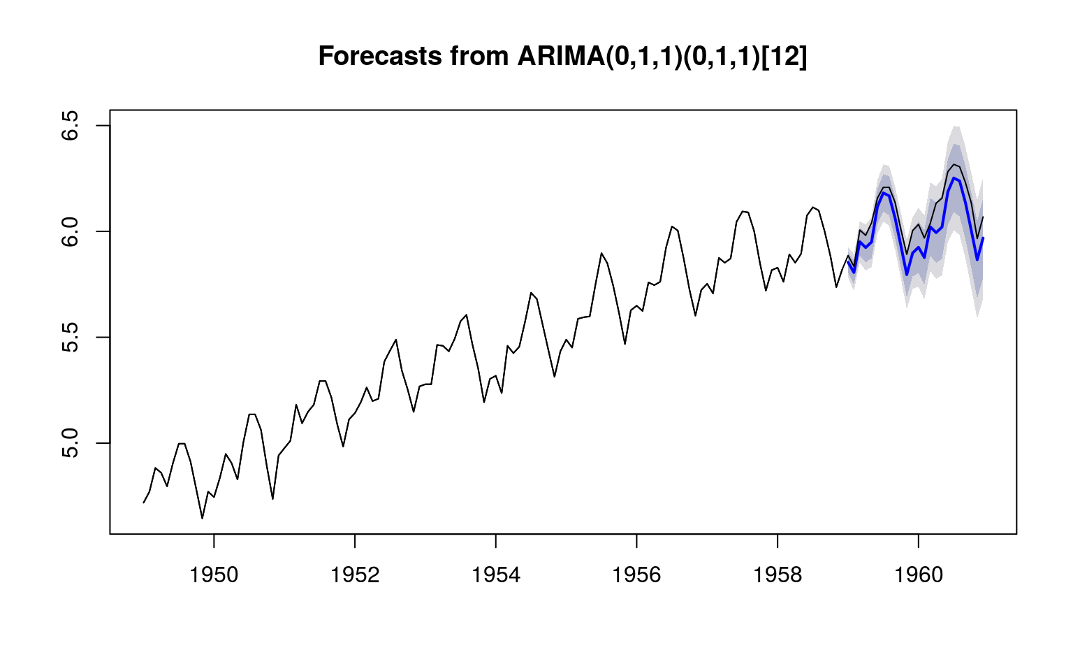
bic -384.1173 -377.0104 -379.4776

模型预测

m1 <- Arima(ap1, order=c(0, 1, 1), seasonal=list(order=c(0, 1, 1), freq=12))
plot(forecast(m1, 24)); lines(ap)

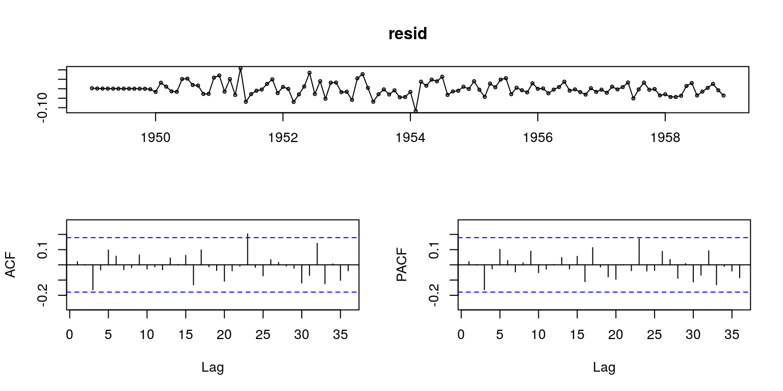
模型诊断: 残差自回归图

残差自回归及偏自回归值基本都不超过置信边界，可认为残差是白噪声(信息提取完全)。

resid <- ap1-m1$fitted
tsdisplay(resid)

模型诊断: Ljung-Box检验

> Box.test(resid, lag=20, type="Ljung-Box")

    Box-Ljung test

data:  resid
X-squared = 12.679, df = 20, p-value = 0.8907

没有证据证明在滞后 1-20 阶中预测误差是非零自相关的，亦即可认为残差是白噪声序列(信息提取完全)。

Thank you!

返回目录

目录

数据结构

ts、xts、zoo类

定距时间序列

不规则时间序列

可视化

时间序列图: plot.ts

时间序列图: plot.xts

时间序列图: quantmod包

时间序列图: dygraphs包

分解时间序列 Decomposition

季节性和非季节数据

季节性数据(1) - decompose移动平均法

季节性数据(2) - 局部加权回归法STL

季节性数据(3) - 调整

非季节性数据

指数平滑法(Exponential Smoothing)

适用条件

简单指数平滑法(1)

简单指数平滑法(2)

简单指数平滑法(3)

Holt指数平滑法(1)

Holt指数平滑法(2)

Holt指数平滑法(3)

Holt-Winters指数平滑法(1)

Holt-Winters指数平滑法(2)

Holt-Winters指数平滑法(3)

ARIMA模型

整合移动平均自回归(ARIMA)模型

差分及增强的Dickey-Fuller单位根检验

ADF平稳性检验

自回归图及偏自回归图

构建Arima模型

Arima(p, d, q)(P, D, Q)m模型选择原则

(P, D, Q)m季节性参数的确定

模型预测

模型诊断: 残差自回归图

模型诊断: Ljung-Box检验

`ts`、`xts`、`zoo`类

时间序列图: `plot.ts`

时间序列图: `plot.xts`

时间序列图: `quantmod`包

时间序列图: `dygraphs`包

季节性数据(1) - `decompose`移动平均法

季节性数据(2) - 局部加权回归法`STL`

指数平滑法
(Exponential Smoothing)

Arima(p, d, q)(P, D, Q)_m模型选择原则

(P, D, Q)_m季节性参数的确定